This article on vectors is part of an ongoing crash course on linear algebra programming, demonstrating concepts and implementations in Python. The following examples will demonstrate some of the algebraic and geometric interpretations of a vector using Python. A vector is an ordered list of numbers, represented in row or column form.
Linear Algebra: Python Series - View all articles in this series.
This small series of articles on linear algebra is meant to help you prepare for learning the deeper concepts related to Machine Learning and math that drives the higher level abstractions provided by many of the libraries available today.
Python examples in this article make use of the Numpy library. Read my article Python Data Essentials - Numpy if you want a quick overview on this important Python library. Visualizations are accomplished with the Matplotlib Python library. For a beginners guide to Matplotlib might try my article Python Data Essentials - Matplotlib and Seaborn
import numpy as np
import matplotlib.pyplot as plt
from mpl_toolkits.mplot3d import Axes3D
§2026 Update
The linear algebra here has not changed. Vectors work the way they always have. A few library details moved on since 2018, so the code below has been brought up to date for current NumPy and Matplotlib.
For 3D plots, create the axis with fig.add_subplot(projection='3d'); the older fig.gca(projection='3d') was removed from Matplotlib, and the from mpl_toolkits.mplot3d import Axes3D import is no longer needed. NumPy 2.0 landed in 2024, but nothing here depends on anything it removed: the array creation, np.dot, np.vstack, and np.pi used in this article all behave the same on 2.x.
If you would rather work through this in Go than Python, I later wrote a Go linear algebra series that covers the same ground with Gonum. Same math, different toolbox.
The article continues below. The 2026 Update above covers what’s changed; the code examples have been updated to run on current NumPy and Matplotlib.
§Algebraic vs Geometric Interpretations
Vectors are a list of numbers containing metrics or coordinates. Both algebraic or geometric intuitions may be used to represent vectors. Each number inside a vector is considered an element and the order of elements in a vector is important. The $\mathbb{R}$ symbol denotes a Real number, and in this example, two real numbers are created with a row vector.
§An $\mathbb{R}^2$ row vector
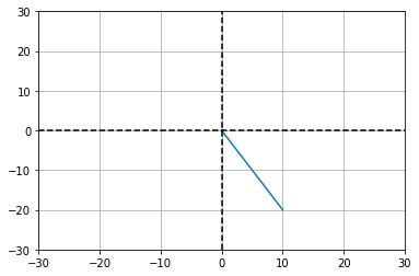
$ \vec{va} = \left[ \begin{array}{ccc} 10 & -20 \ \end{array} \right] $
# a 2-dimensional row vector
va = np.array([ 10, -20 ])

print(f'\n{va}\n')
print(f' type: {type(va)}')
print(f' size: {va.size}')
print(f'shape: {va.shape}')
[ 10 -20]

 type: <class 'numpy.ndarray'>
 size: 2
shape: (2,)
Geometric vectors describe a length and direction. The origin (0,0) is a common starting point for most vectors. However, they may begin anywhere.
# plot the vector in "standard position"
plt.plot([0,va[0]],[0,va[1]])

# create a dotted line from -20 to 20 on 0 x axis
plt.plot([-30, 30],[0, 0],'k--')

# create a dotted line from -20 to 20 on 0 y axis
plt.plot([0, 0],[-30, 30],'k--')

# add some grid lines
plt.grid()

# fit the axis
plt.axis((-30, 30, -30, 30))
plt.show()
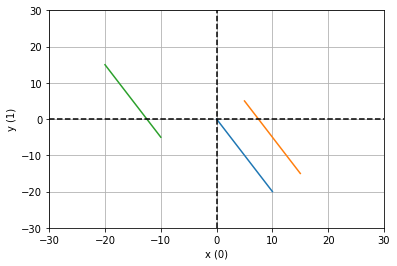
Vectors are robust to translation, meaning that there can be many [ 10 -20] vectors all with different origins. A geometric vector begins at an origin, whereas a coordinate may exist anywhere.
# standard position
sp = np.array([ 0, 0 ])

# position a
pa = np.array([ 5, 5 ])

# position b
pb = np.array([ -20, 15 ])

plt.plot([sp[0],va[0]],[sp[0],va[1]])
plt.plot([pa[0],va[0]+pa[0]],[pa[1],va[1]+pa[1]])
plt.plot([pb[0],va[0]+pb[0]],[pb[1],va[1]+pb[1]])

# create a dotted line from -20 to 20 on 0 x axis
plt.plot([-30, 30],[0, 0],'k--')

# create a dotted line from -20 to 20 on 0 y axis
plt.plot([0, 0],[-30, 30],'k--')

# add some grid lines
plt.grid()

plt.xlabel('x (0)')
plt.ylabel('y (1)')

# fit the axis
plt.axis((-30, 30, -30, 30))
plt.show()
§A 3-dimensional row vector
$ \vec{vb} = \left[ \begin{array}{ccc} 10 & -20 & \pi \ \end{array} \right] $
# a 3-dimensional row vector
vb = np.array([ 10, -20, np.pi ])

print(f'\n{vb}\n')
print(f' type: {type(vb)}')
print(f' size: {vb.size}')
print(f'shape: {vb.shape}')
[ 10.         -20.           3.14159265]

 type: <class 'numpy.ndarray'>
 size: 3
shape: (3,)
# plotting the 3-dimensional vb
fig = plt.figure()
ax = fig.add_subplot(projection='3d')
ax.plot([0, vb[0]],[0, vb[1]],[0, vb[2]])

# add some dashed lines across the x, y and z axis
ax.plot([0, 0],[0, 0],[-20, 20],'k--')
ax.plot([0, 0],[-20, 20],[0, 0],'k--')
ax.plot([-20, 20],[0, 0],[0, 0],'k--')
plt.show()

§A 3-dimensional column vector
$\vec{vb}$ can be transposed $\vec{vb} = \vec{vb}^{T}$ to form a 3-dimensional column vector.
# transposing 1-d vectors is not typically needed
# with numpy as it will automatically broadcast a
# 1D array when doing various calculations
np.vstack(vb)
array([[ 10.  ],
       [-20.  ],
       [  3.14]])
§Addition and Subtraction
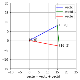
Vector addition and subtraction requires vectors of equal length. Create two $\mathbb{R}2$ (Real number) vectors $\vec{vectc}$ and $\vec{vectd}$.
- Add the vectors together $\vec{vecte} = \vec{vectc} + \vec{vectd}$
- Subtract c from d, $\vec{vectf} = \vec{vectc} - \vec{vectd}$
# two R2 vectors
vectc = np.array([ 15, 8 ])
vectd = np.array([ 1,  -11 ])

# add the vectors
vecte = vectc + vectd
vecte
array([16, -3])
# geometric intuition
fig, ax = plt.subplots()

ax.annotate([0,0], (0,0))
ax.annotate(vectc, vectc)
ax.annotate(vecte, vecte)

ax.plot([0, vectc[0]],[0, vectc[1]],'b',label='vectc')
ax.plot([vectc[0], vectc[0]+vectd[0]],[vectc[1], vectc[1]+vectd[1]],'g',label='vectd')
ax.plot([0, vecte[0]],[0, vecte[1]],'r',label='vecte')

ax.axis('square')
ax.axis((-10, 25, -15, 20 ))
ax.grid()
plt.legend()
plt.xlabel('vecte = vectc + vectd')
plt.show()
An algebraic interpretation:
# subtract d from c
vectf = vectc - vectd
vectf
array([14, 19])
§Scalar Multiplication
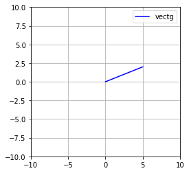
Create $\vec{vectg}$ as an $\mathbb{R}2$ array with coordinates [ 5, 2 ]
vectg = np.array([ 5, 2 ])

# geometric intuition
fig, ax = plt.subplots()
ax.plot([0, vectg[0]],[0, vectg[1]],'b',label='vectg')
ax.grid()
ax.axis('square')
ax.axis((-10, 10, -10, 10 ))
plt.legend()
plt.show()
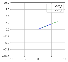
Scalars are often noted with lowercase greek symbols like alpha: $\alpha$, beta: $\beta$, and theta: $\theta$
$\vec{vecth} = \theta\vec{vectg}$
m = 1.5
vecth = vectg * m
vecth
array([ 7.5, 3. ])
A geometric intrepretation shows the scaling of the vector through multiplication, changing its length while its origin remains constant.
# geometric intuition
fig, ax = plt.subplots()
ax.plot([0, vectg[0]],[0, vectg[1]],'b',label='vect_g')
ax.plot([0, vecth[0]],[0, vecth[1]],'g:',label='vect_h')
ax.grid()
ax.axis('square')
ax.axis((-10, 10, -10, 10 ))
plt.legend()
plt.show()
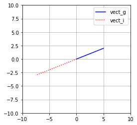
Multiply $\vec{vectg}$ by the scalar m2.
$\vec{vecti} = \vec{vectg}\alpha$
alpha = -1.5

vecti = vectg * alpha

# geometric intuition
fig, ax = plt.subplots()
ax.plot([0, vectg[0]],[0, vectg[1]],'b',label='vect_g')
ax.plot([0, vecti[0]],[0, vecti[1]],'r:',label='vect_i')
ax.grid()
ax.axis('square')
ax.axis((-10, 10, -10, 10 ))
plt.legend()
plt.show()
§Vector multiplication (dot product)
The dot product (or scalar product) is a single number representing the relationship between two vectors.
- $\vec{vectr}$ is an $\mathbb{R}3$ array with coordinates [ 2, 5, -7 ]
- $\vec{vects}$ is an $\mathbb{R}3$ array with coordinates [ 1.5, 4, -1 ]
- The dot product of $\vec{vectr}$ and $\vec{vects}$ is 30.
- $\vec{vectr}\cdot\vec{vects} = \vec{vectr}^T\vec{vects} = \sum_{i=1}^n\vec{vectr_i}\vec{vects_i}$
vectr = np.array([ 2, 5, -7])
vects = np.array([ 1.5, 4, -1])

# the dot product is the sum of products
rs = np.dot(vectr,vects)
rs
30.0
§Next: Matrices
Check out the next article in this series, Linear Algebra: Matrices 1: Linear Algebra Crash Course for Programmers Part 2a.
Linear Algebra: Python Series - View all articles in this series.