Linear Algebra: Matrices 1

This article on matrices is part two of an ongoing crash course on programming with linear algebra, demonstrating concepts and implementations in Python. The following examples will demonstrate some of the various mathematical notations and their corresponding implementations, easily translatable to any programming language with mature math libraries.

This series began with Linear Algebra: Vectors Crash Course for Python Programmers Part 1. Vectors are the building blocks of matrices, and a good foundational understanding of vectors is essential to understanding matrices.

This article covers some matrix notation, common matrix types, methods of addition and multiplication and rank. Future articles will cover additional concepts.

This small series of articles on linear algebra is meant to help in preparation for learning the more profound concepts related to Machine Learning, AI and math that drives the higher level abstractions provided by many of the libraries available today.

Python examples in this article make use of the Numpy library. Read the article Python Data Essentials - Numpy if you want a quick overview of this important Python library along with the Matplotlib Python library for visualizations. For a beginners guide to Matplotlib might try my article Python Data Essentials - Matplotlib and Seaborn

import numpy as np
import matplotlib.pyplot as plt
import math
from mpl_toolkits.mplot3d import Axes3D
import seaborn as sb

%matplotlib inline

Support this blog! Buy my new book:

Advanced Platform Development with Kubernetes

What You'll Learn

Build data pipelines with MQTT, NiFi, Logstash, MinIO, Hive, Presto, Kafka and Elasticsearch
Leverage Serverless ETL with OpenFaaS
Explore Blockchain networking with Ethereum
Support a multi-tenant Data Science platform with JupyterHub, MLflow and Seldon Core
Build a Multi-cloud, Hybrid cluster, securely bridging on-premise and cloud-based Kubernetes nodes

Matrix Notation

It is common to note a matrix with a capital letter. The following is a three by two matrix of Real numbers.

$ \boldsymbol{A} = \begin{pmatrix} 10 & 5 \\ -20 & 2 \\ \pi & 1.5 \\ \end{pmatrix} = \begin{bmatrix} 10 & 5 \\ -20 & 2 \\ \pi & 1.5 \\ \end{bmatrix} = \begin{matrix} 10 & 5 \\ -20 & 2 \\ \pi & 1.5 \\ \end{matrix} = \mathbb{R}^{3\times2} $

# python matrix 
c = np.array([[10,5],[-20,2],[np.pi,1.5]])
c

array([[ 10.        ,   5.        ],
       [-20.        ,   2.        ],
       [  3.14159265,   1.5       ]])

Matrix dimensions are noted by row first and then column. The matrix $\boldsymbol{D}^{3\times4}$ contains three rows and four columns.

$ \boldsymbol{D} = \begin{pmatrix} 10 & 5 & 2 & 1 \\ -20 & 2 & 3 & 6.6 \\ \pi & 1.5 & 2 & 0 \\ \end{pmatrix} = \mathbb{R}^{3\times4} $

Accessing Elements

Subscript numbers represent an element in a matrix by row and column. Access elements of the matrix $\boldsymbol{D}$ with the notation $d_{ij}$ where ${i}$ is the row and ${j}$ is the column.

$ {d}_{2,4} = 6.6 $

d = np.array([[10,5,2,1],[-20,2,3,6.6],[np.pi,1.5,2,0]])
d

array([[ 10.        ,   5.        ,   2.        ,   1.        ],
       [-20.        ,   2.        ,   3.        ,   6.6       ],
       [  3.14159265,   1.5       ,   2.        ,   0.        ]])

Python, like many computer languages, starts indexing at zero. The example below implements ${d}_{2,4} = 6.6$ in Python.

d[1][3]

6.5999999999999996

Common Matrix Types

The following section describes a hand full of matrix types.

Square and Rectangular Matrices

Matricies are Square (${m} = {n}$) or Rectangular (${m} \neq {n}$)

The following is a square matrix of fives, where ${m}=2$ and ${n}=2$:

$ \boldsymbol{L} = \begin{pmatrix} 5 & 5 \\ 5 & 5 \\ \end{pmatrix} = \mathbb{R}^{2\times2} $

# numpy.full(shape, fill_value, dtype=None, order='C')[source]
# Returns a new array of given shape and type, filled with fill_value.
l = np.full((2,2), 5)
l

array([[5, 5],
       [5, 5]])

The following is a rectangular matrix $\boldsymbol{P}_{3,2}$ of fours, where ${m}=3$ and ${n}=2$:

$ \boldsymbol{P} = \begin{pmatrix} 4 & 4 \\ 4 & 4 \\ 4 & 4 \\ \end{pmatrix} = \mathbb{R}^{3\times2} $

p = np.full((3,2), 4)
p

array([[4, 4],
       [4, 4],
       [4, 4]])

Zero (null) Matricies

A Zero matrix only contains zeros and may be square (${m} = {n}$) or rectangular (${m} \neq {n}$).

$ \boldsymbol{Z} = \begin{pmatrix} 0 & 0 \\ 0 & 0 \\ \end{pmatrix} = \mathbb{R}^{2\times2} $

np.zeros((2,2))

array([[ 0.,  0.],
       [ 0.,  0.]])

Diagonal Matricies

Diagonal matrices may be Square or Rectangular contain only zeros for off-diagonal entries, however, elements in the main diagonal are unrestricted and may also be zero.

$ \boldsymbol{W} = \begin{pmatrix} 2 & 0 & 0 & 0 & 0 \\ 0 & 3 & 0 & 0 & 0 \\ 0 & 0 & 5 & 0 & 0 \\ 0 & 0 & 0 & 7 & 0 \\ 0 & 0 & 0 & 0 & 9 \\ \end{pmatrix} = \mathbb{R}^{5\times5} $

The above matrix $\boldsymbol{W}$ is diagonal in that every ${w}_{i}$ row and $w_{ij}$ column in the range $1, 2, \ldots, n$ where $i \ne j$ then $w_{i,j} = 0$.

$\forall i,j \in {1, 2, \ldots, n}, i \ne j \implies w_{i,j} = 0$

# create the square diagonal matrix W 
w = np.diag([2,3,5,7,9])
w

array([[2, 0, 0, 0, 0],
       [0, 3, 0, 0, 0],
       [0, 0, 5, 0, 0],
       [0, 0, 0, 7, 0],
       [0, 0, 0, 0, 9]])

w.shape

(5, 5)

Diagonal elements in a rectangular matrix.

$ \boldsymbol{G} = \begin{pmatrix} 2 & 0 & 0 & 0 & 0 & 0 \\ 0 & 3 & 0 & 0 & 0 & 0 \\ 0 & 0 & 5 & 0 & 0 & 0 \\ 0 & 0 & 0 & 7 & 0 & 0 \\ 0 & 0 & 0 & 0 & 9 & 0 \\ \end{pmatrix} = \mathbb{R}^{5\times6} $

# Create the rectangular diagonal matrix G
# by appending a column vector of zeros
cz = np.full((w.shape[0],1), 0)

# by appending a column by axis=1
g = np.append(w, cz, axis=1)
g

array([[2, 0, 0, 0, 0, 0],
       [0, 3, 0, 0, 0, 0],
       [0, 0, 5, 0, 0, 0],
       [0, 0, 0, 7, 0, 0],
       [0, 0, 0, 0, 9, 0]])

g.shape

(5, 6)

Identity Matricies

Identity matricies are square (${m} = {n}$) and contain ones across the diagonal with zeros elsewhere. Identity matricies are noted with the symbol $\boldsymbol{I}$

$ \boldsymbol{I} = \begin{pmatrix} 1 & 0 & 0 \\ 0 & \ddots & 0 \\ 0 & 0 & 1 \\ \end{pmatrix} $

$\forall i,j \in {1, 2, \ldots, n}, i \ne j \implies w_{i,j} = 0$

$\forall i,j \in {1, 2, \ldots, n}, i = j \implies w_{i,j} = 1$

eye = np.eye(5)
eye

array([[ 1.,  0.,  0.,  0.,  0.],
       [ 0.,  1.,  0.,  0.,  0.],
       [ 0.,  0.,  1.,  0.,  0.],
       [ 0.,  0.,  0.,  1.,  0.],
       [ 0.,  0.,  0.,  0.,  1.]])

It is common to see a constant value next to the identity matrix symbol $\boldsymbol{I}$ such as $5\boldsymbol{I}$.

$ 5\boldsymbol{I} = \begin{pmatrix} 5 & 0 & 0 \\ 0 & \ddots & 0 \\ 0 & 0 & 5 \\ \end{pmatrix} $

5 * eye

array([[ 5.,  0.,  0.,  0.,  0.],
       [ 0.,  5.,  0.,  0.,  0.],
       [ 0.,  0.,  5.,  0.,  0.],
       [ 0.,  0.,  0.,  5.,  0.],
       [ 0.,  0.,  0.,  0.,  5.]])

Triangular Matricies

Triangular matrices are categorized as upper or lower with zeros above or below the diagonal.

Upper triangular matrix:

$ \boldsymbol{U} = \begin{pmatrix} 1 & 2 & 3 \\ 0 & 5 & 6 \\ 0 & 0 & 9 \\ \end{pmatrix} $

Lower triangular matrix:

$ \boldsymbol{L} = \begin{pmatrix} 1 & 0 & 0 \\ 4 & 5 & 0 \\ 7 & 8 & 9 \\ \end{pmatrix} $

# create an array of numbers, 1...9
nums = np.arange(1,10)
nums

array([1, 2, 3, 4, 5, 6, 7, 8, 9])

# reshape the array into a 3x3 matrix
mx = np.reshape(nums, (3,3))
mx

array([[1, 2, 3],
       [4, 5, 6],
       [7, 8, 9]])

# create an upper triangular matrix
u = np.triu(mx)
print(f'matrix U:\n{u}')

matrix U:
[[1 2 3]
 [0 5 6]
 [0 0 9]]

# create a lower triangular matrix
l = np.tril(mx)
print(f'matrix L:\n{l}')

matrix L:
[[1 0 0]
 [4 5 0]
 [7 8 9]]

Transposed Matrix

Transposing flips a matrix over its diagonal. A transposed matrix may be noted as $\boldsymbol{I}^T$ or $\boldsymbol{I}'$. Transposing is easy to see when using one of the triangular matrices above.

Lower triangular matrix:

$ \boldsymbol{L} = \begin{pmatrix} 1 & 0 & 0 \\ 4 & 5 & 0 \\ 7 & 8 & 9 \\ \end{pmatrix} $

Transposed:

$ \boldsymbol{L}^T = \begin{pmatrix} 1 & 4 & 7 \\ 0 & 5 & 8 \\ 0 & 0 & 9 \\ \end{pmatrix} $

Every i-th row, j-th column have been transposed:

$\boldsymbol{L}^T_{i j} = \boldsymbol{L}_{j i}$

print(f'matrix L:\n{l}')

matrix L:
[[1 0 0]
 [4 5 0]
 [7 8 9]]

# note: zero based index
# i (row 3) and j (colum 1) 
l[2][0]

# transpose L (also. np.transpose(l))
l.T

array([[1, 4, 7],
       [0, 5, 8],
       [0, 0, 9]])

# i (row 1) and j (colum 3) 
l.T[0][2]

Symmetric & Skew-symetric Matricies

Symmetric & Skew-symetric matricies have values that correlate to the transposed position above and below the diagonal. A symmetrical matrix can be expressed as $\boldsymbol{V}^T = \boldsymbol{V}$. A skew-symetric matrix can be expressed as $\boldsymbol{W}^T = -\boldsymbol{W}$.

# Using the upper triangle matrix from above 
u

array([[1, 2, 3],
       [0, 5, 6],
       [0, 0, 9]])

$\boldsymbol{S} = \boldsymbol{U} + \boldsymbol{U}^T$

# Add the upper triangle matrix to a transposed
# version of itself. We are not concerned with the diagonal.
s = u + u.T
print(f'matrix S:\n{s}')

matrix S:
[[ 2  2  3]
 [ 2 10  6]
 [ 3  6 18]]

Check the matrix $\boldsymbol{S}$ for symmetry. Does $\boldsymbol{S}^T = \boldsymbol{S}$ ?

# is the s matrix is symmetric
np.array_equal(s, s.T)

True

Another method for creating a symmetric matrix involves multiplying a matrix by its transpose.

$\boldsymbol{G} = \begin{pmatrix} 1 & 2 & 3 \\ 4 & 5 & 6 \\ 7 & 8 & 9 \\ \end{pmatrix} $

$\boldsymbol{G}\boldsymbol{G}^T = \underbrace{ \begin{pmatrix} 14 & \boldsymbol{32} & \boldsymbol{50} \\ \boldsymbol{32} & 77 & \boldsymbol{122} \\ \boldsymbol{50} & \boldsymbol{122} & 194 \\ \end{pmatrix}}_{symmetric} $

G = np.arange(1,10).reshape(3,3)

G @ G.T

array([[ 14,  32,  50],
       [ 32,  77, 122],
       [ 50, 122, 194]])

Next, create a skew-symmetric matrix by using the same upper triangle matrix, and creating a transposed additive inverse of it, then add the two matrices together.

$\boldsymbol{V} = -\boldsymbol{U} + \boldsymbol{U}^T$

v = (u * -1) + u.T
print(f'matrix V:\n{v}')

matrix V:
[[ 0 -2 -3]
 [ 2  0 -6]
 [ 3  6  0]]

Check for skew-symmertic $\boldsymbol{V}^T = -\boldsymbol{V}$

# is the s matrix skew-symmetric?
np.array_equal(v.T, (v * -1))

True

Augmented Matricies

Augmented matrices often used for solving a system of equations, they are the concatenation of two matrices with the same number of rows (${m} = {m}$).

$ \boldsymbol{A} = \begin{pmatrix} 1 & 0 & 0 \\ 4 & 5 & 0 \\ 7 & 8 & 9 \\ \end{pmatrix} \sqcup \begin{pmatrix} 1 & 4 & 7 \\ 0 & 5 & 8 \\ 0 & 0 & 9 \\ \end{pmatrix} = \left( \begin{array}{ccc|ccc} 1 & 0 & 0 & 1 & 4 & 7 \\ 4 & 5 & 0 & 0 & 5 & 8 \\ 7 & 8 & 9 & 0 & 0 & 9 \\ \end{array} \right) $

print(f'matrix L:\n{l}\n')
print(f'matrix U:\n{u}')

matrix L:
[[1 0 0]
 [4 5 0]
 [7 8 9]]

matrix U:
[[1 2 3]
 [0 5 6]
 [0 0 9]]

a = np.append(l, u, axis=1)
print(f'Augmented matrix A:\n{a}')

Augmented matrix A:
[[1 0 0 1 2 3]
 [4 5 0 0 5 6]
 [7 8 9 0 0 9]]

Complex Matricies

Complex matricies, often noted as $\mathbb{C}$, contain complex numbers.

# create a zero matrix of the data type np.complex
p = np.zeros((3,3), dtype=np.complex)
p[0][1] = 1 + 1 + 7j
print(f'Complex matrix P:\n{p}')

Complex matrix P:
[[ 0.+0.j  2.+7.j  0.+0.j]
 [ 0.+0.j  0.+0.j  0.+0.j]
 [ 0.+0.j  0.+0.j  0.+0.j]]

p[0][0]

0j

Matrix Addition

Matrix addition and subtraction works only with matrices of equal size (m by n). The entrywise sum is calculated by adding each value ${ij}$ of one matrix to the corresponding ${ij}$ of the other. Matrix addition is commutative and associative, for instance, the following are valid:

$ \boldsymbol{G} = \begin{pmatrix} 1 & 2 \\ 3 & 4 \\ \end{pmatrix} , \boldsymbol{H} = \begin{pmatrix} 2 & 3 \\ 3 & 3 \\ \end{pmatrix} , \boldsymbol{F} = \begin{pmatrix} 5 & 4 \\ 3 & -1 \\ \end{pmatrix} $

$\boldsymbol{G} + \boldsymbol{H} = \boldsymbol{H} + \boldsymbol{G} = \begin{pmatrix} 3 & 5 \\ 6 & 7 \\ \end{pmatrix} $

$\boldsymbol{G} + (\boldsymbol{H} + \boldsymbol{F}) = (\boldsymbol{G} + \boldsymbol{H}) + \boldsymbol{F} = \begin{pmatrix} 8 & 9 \\ 9 & 6 \\ \end{pmatrix} $

There are other types of matrix addition opperations including Direct Sum and Kronecker sum.

# construct a 2x2 matrix by reshaping a 1x4 array
g = np.array([1,2,3,4]).reshape(2,2)
g

array([[1, 2],
       [3, 4]])

h = np.array([2,3,3,3]).reshape(2,2)
h

array([[2, 3],
       [3, 3]])

f = np.array([5,4,3,-1]).reshape(2,2)
f

array([[ 5,  4],
       [ 3, -1]])

g + h == h + g

array([[ True,  True],
       [ True,  True]], dtype=bool)

if (g + h == h + g).all:
    print("equasions are commutative")

equations are commutative

if (g + ( h + f ) == (g + h) + f).all:
    print("equasions are associative")

equations are associative

g - h == h - g

array([[False, False],
       [ True, False]], dtype=bool)

Matrix Scalar Multiplication

Multiplying a scalar by a matrix multiplies each ${ij}$ element by the scalar.

$\theta \begin{pmatrix} {a} & {b}\\ {c} & {d} \\ \end{pmatrix} = \begin{pmatrix} \theta{a} & \theta{b}\\ \theta{c} & \theta{d} \\ \end{pmatrix} $

Scalar multiplication is commutative.

$\boldsymbol{G}\theta = \theta\boldsymbol{G}$

$ \begin{pmatrix} \theta{a} & \theta{b}\\ \theta{c} & \theta{d} \\ \end{pmatrix} = \begin{pmatrix} {a} & {b}\\ {c} & {d} \\ \end{pmatrix} \theta $

theta = 5
g * theta

array([[ 5, 10],
       [15, 20]])

theta * g

array([[ 5, 10],
       [15, 20]])

Trace

The trace of a matrix is the sum of the diagonal of a square ${n}$ x ${n}$ matrix, $\sum_{i=1}^n{a}_{ii}$.

$\mathrm{tr}\left(\boldsymbol{A}\right) = \sum_{i=1}^n \begin{pmatrix} \boldsymbol{1} & 2 & 3 \\ 4 & \boldsymbol{5} & 6 \\ 7 & 8 & \boldsymbol{9} \\ \end{pmatrix}_{ii} = 15 $

a = np.array([1,2,3,4,5,6,7,8,9]).reshape(3,3)
a

array([[1, 2, 3],
       [4, 5, 6],
       [7, 8, 9]])

# use Numpy trace function
np.trace(a)

# extract and diagonal and sum
np.diag(a).sum()

Matrix Multiplication

Matrix multiplication is associative and generaly non-commutative.

Standard Matrix Multiplication

Left multiplies right, for example $\boldsymbol{T}\boldsymbol{U}$, $\boldsymbol{T}$ multiplies $\boldsymbol{U}$. Valid standard matrix multiplication requires the inner dimensions be the same, for instance, the number of columns (${n}$) in the left matrix must match the number of rows (${m}$) in the left matrix.

$\boldsymbol{T} = \begin{pmatrix} 1 & 2 & 3 \\ 4 & 5 & 6 \\ 7 & 8 & 9 \\ 10 & 11 & 12 \\ \end{pmatrix} = \mathbb{R}^{4\times\boldsymbol{3}} $

$\boldsymbol{U} = \begin{pmatrix} -2 & 4 \\ -6 & 8 \\ -10 & 12 \\ \end{pmatrix} = \mathbb{R}^{\boldsymbol{3}\times{2}} $

$\boldsymbol{T}_{n} = \boldsymbol{U}_{m}$

The product matrix produced when multiplying ${\boldsymbol{T}}^{\boldsymbol{4}x3}$ ${\boldsymbol{U}^{3x\boldsymbol{2}}}$ will have the size $m = {4}$ , n = ${2}$

# create a range from 1 to 12 and reshape it into
# a 4x3 matrix
t = np.arange(1,13).reshape(4,3)
t

array([[ 1,  2,  3],
       [ 4,  5,  6],
       [ 7,  8,  9],
       [10, 11, 12]])

Next, we can construct the $\boldsymbol{U}$ matrix by using a list compreshesion in Python.

# create a range in steps of 2 from 2 to 12
u = np.arange(2,14,2)

# use a list comprehension to convert every other
# index in the array to a nagative
u = [ i if idx % 2 else i * -1 for idx, i in enumerate(u)]
u = np.array(u).reshape(3,2)
u

array([[ -2,   4],
       [ -6,   8],
       [-10,  12]])

t.shape

(4, 3)

u.shape

(3, 2)

d = np.matmul(t,u)
d

array([[ -44,   56],
       [ -98,  128],
       [-152,  200],
       [-206,  272]])

# alternative
t @ u

array([[ -44,   56],
       [ -98,  128],
       [-152,  200],
       [-206,  272]])

d.shape

(4, 2)

# The @ operator calls the array's __matmul__ method
t @ u

array([[ -44,   56],
       [ -98,  128],
       [-152,  200],
       [-206,  272]])

Vector Dot Product

Matrix vector products will always be a row or column vector.

$ \begin{pmatrix} a_{11} & a_{12} & a_{13} \\ a_{21} & a_{22} & a_{23} \\ a_{31} & a_{32} & a_{33} \\ a_{41} & a_{42} & a_{43} \\ \end{pmatrix} \begin{bmatrix} x_1 \\ x_2 \\ x_3 \\ \end{bmatrix} = \begin{bmatrix} a_{11}x_1 + a_{12}x_2 + a_{13}x_3 \\ a_{21}x_1 + a_{22}x_2 + a_{23}x_3 \\ a_{31}x_1 + a_{32}x_2 + a_{33}x_3 \\ a_{41}x_1 + a_{42}x_2 + a_{43}x_3 \\ \end{bmatrix} = \begin{bmatrix} b_1 \\ b_2 \\ b_3 \\ b_4 \\ \end{bmatrix} $

$ \underbrace{ \begin{pmatrix} 2 & 4 & 6 \\ 8 & 10 & 12 \\ 14 & 16 & 18 \\ 20 & 22 & 24 \\ \end{pmatrix}}_{\boldsymbol{A}} \underbrace{ \begin{bmatrix} 1.5 \\ 1 \\ .5 \\ \end{bmatrix} }_{\vec{x}} = \underbrace{ \begin{bmatrix} 10 \\ 28 \\ 46 \\ 64 \\ \end{bmatrix} }_{\boldsymbol{A}\vec{x}} $

a = np.matrix(np.arange(2,26,2).reshape(4,3))
a

matrix([[ 2,  4,  6],
        [ 8, 10, 12],
        [14, 16, 18],
        [20, 22, 24]])

x = np.matrix(np.flip(np.arange(.5,2,.5), axis=0)).T
x

matrix([[ 1.5],
        [ 1. ],
        [ 0.5]])

# vector dot product
b = a @ x
b

matrix([[ 10.],
        [ 28.],
        [ 46.],
        [ 64.]])

d = np.matrix(np.arange(1,6).reshape(1,5))
d

matrix([[1, 2, 3, 4, 5]])

w = np.matrix(np.arange(1,6).reshape(5,1))
w

matrix([[1],
        [2],
        [3],
        [4],
        [5]])

d @ w

matrix([[55]])

w @ d

matrix([[ 1,  2,  3,  4,  5],
        [ 2,  4,  6,  8, 10],
        [ 3,  6,  9, 12, 15],
        [ 4,  8, 12, 16, 20],
        [ 5, 10, 15, 20, 25]])

Matrix-Vector Multiplication

The result of multiplying a vector by a matrix or a matrix by a vector will always be a vector.

$ \begin{pmatrix} a & b & c \\ d & e & f \\ g & h & i \\ \end{pmatrix} \vec{ \begin{bmatrix} 2 \\ 3 \\ 4 \\ \end{bmatrix}} = \vec{ \begin{bmatrix} 2a+3b+4c \\ 2d+3e+4f \\ 2g+3h+4i \\ \end{bmatrix} } $

$ \vec{ \begin{bmatrix} 2 & 3 & 4 \\ \end{bmatrix} } \begin{pmatrix} a & b & c \\ d & e & f \\ g & h & i \\ \end{pmatrix} = \vec{ \begin{bmatrix} 2a+3d+4g \\ 2b+3e+4h \\ 2c+3f+4i \\ \end{bmatrix} } $

# construct a column vector with numpy using octave / matlab style 
v = np.matrix('2; 3; 4')
v

matrix([[2],
        [3],
        [4]])

a = np.arange(1,10).reshape(3,3)
a

array([[1, 2, 3],
       [4, 5, 6],
       [7, 8, 9]])

a * v

matrix([[20],
        [47],
        [74]])

# transpose column vector v into a row vector
v.T * a

matrix([[42, 51, 60]])

Geometric Vector Transformation

The following examples demonstrate 2d and 3d transformations.

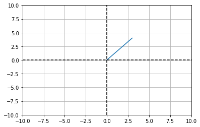
2d Transformation

Transforming a 2d vector with a 2x2 matrix:

$ \begin{pmatrix} 1 & -2 \\ 3 & -1.5 \\ \end{pmatrix} \vec{\begin{bmatrix} 3 \\ 4 \\ \end{bmatrix}} = \vec{\begin{bmatrix} (3\times{1})+(4\times{-2}) \\ (3\times{3})+(4\times{-1.5})\\ \end{bmatrix}} = \vec{\begin{bmatrix} -5\\ 3\\ \end{bmatrix}} $

(3 * 1) + (4 * -2)

-5

# a vector at position 3, 4
v = np.matrix('3 ;4')
v

matrix([[3],
        [4]])

# plot the vector v in "standard position"
plt.plot([0,v[0]],[0,v[1]])

# create a dashed line in the x axis
plt.plot([-10, 10],[0, 0],'k--')

# create a dashed line in the y axis
plt.plot([0, 0],[-10, 10],'k--')

# add some grid lines
plt.grid()

# fit the axis
plt.axis((-10, 10, -10, 10))
plt.show()

png

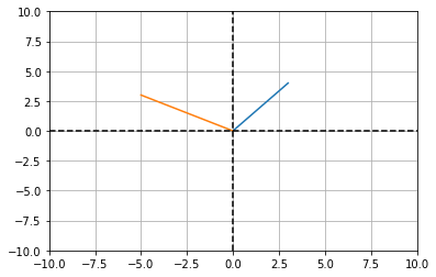
# create a matrix to be used in transforming the vector v
a = np.matrix('1 -2; 3 -1.5')
c = a @ v
c

matrix([[-5.],
        [ 3.]])

# plot the vectors c and c in "standard position"
plt.plot([0,v[0]],[0,v[1]])
plt.plot([0,c[0]],[0,c[1]])

# create a dashed lines
plt.plot([-10, 10],[0, 0],'k--')
plt.plot([0, 0],[-10, 10],'k--')

# add some grid lines
plt.grid()

# fit the axis
plt.axis((-10, 10, -10, 10))
plt.show()

png

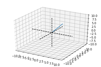
3d Transformation

Next, transform a 3d vector with a 3x3 matrix:

$ \begin{pmatrix} 1 & -4 & .5 \\ 3 & -1.5 & 1.25 \\ -1 & .5 & -.5 \\ \end{pmatrix} \vec{\begin{bmatrix} 3 \\ 4 \\ 5 \\ \end{bmatrix}} = \vec{\begin{bmatrix} (3\times{1})+(4\times{-2})+(5\times{.5}) \\ (3\times{3})+(4\times{-1.5})+(5\times{1.25}) \\ (3\times{-1})+(4\times{.5})+(5\times{-.5}) \\ \end{bmatrix}} = \vec{\begin{bmatrix} -10.5\\ 9.25\\ -3.5 \end{bmatrix}} $

# a vector at position 3, 4, 5
v = np.matrix('3 ;4; 5')
v

matrix([[3],
        [4],
        [5]])

# plotting the 3-dimensional vector from the
# standard position 0,0,0
fig = plt.figure()
ax = fig.gca(projection='3d')
ax.plot([0, v[0]],[0, v[1]],[0, v[2]])

# add some dashed lines across the x, y and z axis
ax.plot([0, 0],[0, 0],[-10, 10],'k--')
ax.plot([0, 0],[-10, 10],[0, 0],'k--')
ax.plot([-10, 10],[0, 0],[0, 0],'k--')
plt.show()

png

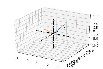
b = np.matrix('1 -4 .5; 3 -1.5 1.25; -1 .5 -.5')
b

matrix([[ 1.  , -4.  ,  0.5 ],
        [ 3.  , -1.5 ,  1.25],
        [-1.  ,  0.5 , -0.5 ]])

c = b @ v
c

matrix([[-10.5 ],
        [  9.25],
        [ -3.5 ]])

# plotting the 3-dimensional vector from the
# standard position 0,0,0
fig = plt.figure()
ax = fig.gca(projection='3d')
ax.plot([0, v[0]],[0, v[1]],[0, v[2]])
ax.plot([0, c[0]],[0, c[1]],[0, c[2]])

# add some dashed lines across the x, y and z axis
ax.plot([0, 0],[0, 0],[-10, 10],'k--')
ax.plot([0, 0],[-10, 10],[0, 0],'k--')
ax.plot([-10, 10],[0, 0],[0, 0],'k--')
plt.show()

png

Multiplication with a Diagonal Matrix

When a regular matrix ($\boldsymbol{F}$) multiplies a diagonal matrix ($\boldsymbol{D}$), it has the effect multiplying each column by the non-zero value in the corresponding diagonal matrix column.

$ \underbrace{\begin{pmatrix} 1 & 2 & 3 \\ 4 & 5 & 6 \\ 7 & 8 & 9 \\ \end{pmatrix}}_{\boldsymbol{F}} \underbrace{\begin{pmatrix} \boldsymbol{t} & 0 & 0 \\ 0 & \boldsymbol{u} & 0 \\ 0 & 0 & \boldsymbol{v} \\ \end{pmatrix}}_{\boldsymbol{D}} = { \begin{pmatrix} \boldsymbol{t}1 & \boldsymbol{u}2 & \boldsymbol{v}3 \\ \boldsymbol{t}4 & \boldsymbol{u}5 & \boldsymbol{v}6 \\ \boldsymbol{t}7 & \boldsymbol{u}8 & \boldsymbol{v}9 \\ \end{pmatrix} } $

When a diagonal matrix ($\boldsymbol{D}$) multiplies a regular matrix ($\boldsymbol{F}$), it has the effect multiplying each row by the non-zero value in the corresponding diagonal matrix row.

$ \underbrace{\begin{pmatrix} \boldsymbol{t} & 0 & 0 \\ 0 & \boldsymbol{u} & 0 \\ 0 & 0 & \boldsymbol{v} \\ \end{pmatrix}}_{\boldsymbol{D}} \underbrace{\begin{pmatrix} 1 & 2 & 3 \\ 4 & 5 & 6 \\ 7 & 8 & 9 \\ \end{pmatrix}}_{\boldsymbol{F}} = {\begin{pmatrix} \boldsymbol{t}1 & \boldsymbol{t}2 & \boldsymbol{t}3 \\ \boldsymbol{u}4 & \boldsymbol{u}5 & \boldsymbol{u}6 \\ \boldsymbol{v}7 & \boldsymbol{v}8 & \boldsymbol{v}9 \\ \end{pmatrix}} $

# create a 3x3 matrix with values from 1 to 10
f = np.arange(1,10).reshape(3,3)
f

array([[1, 2, 3],
       [4, 5, 6],
       [7, 8, 9]])

# create a diagonal matrix 
d = np.diag([2,4,5])
d

array([[2, 0, 0],
       [0, 4, 0],
       [0, 0, 5]])

d @ f

array([[ 2,  4,  6],
       [16, 20, 24],
       [35, 40, 45]])

f @ d

array([[ 2,  8, 15],
       [ 8, 20, 30],
       [14, 32, 45]])

Order of Operations

Reverse the matrix order when operating (such as transpose) on multiplied matrices.

$\boldsymbol{X} = (\boldsymbol{A}\boldsymbol{B}\boldsymbol{C})^T = \boldsymbol{C}^T\boldsymbol{B}^T\boldsymbol{A}^T$

# create 3, 3x3 matricies using octave/matlab style notation
a = np.matrix('1 2 3; 4 5 6; 7 8 9')
b = np.matrix('4 2 1; 7 8 2; 1 2 3')
c = np.matrix('5 4 3; 2 1 2; 3 4 5')
print(f'matrix A =\n{a}\n\nmatrix B =\n{b}\n\nmatrix C =\n{c}\n')

matrix A =
[[1 2 3]
 [4 5 6]
 [7 8 9]]

matrix B =
[[4 2 1]
 [7 8 2]
 [1 2 3]]

matrix C =
[[5 4 3]
 [2 1 2]
 [3 4 5]]

x = (a * b * c).T
x

matrix([[195, 501, 807],
        [164, 416, 668],
        [181, 451, 721]])

np.array_equal(x, (a.T * b.T * c.T))

False

np.array_equal(x, (c.T * b.T * a.T))

True

Hadamard Multiplication (element-wise)

Hadamard multiplication multiplies an element in the first matrix by the corresponding element in another. The Hadamard product is commutative, associative and distributive.

$\underbrace{ \begin{pmatrix} a_{11} & a_{12} \\ a_{21} & a_{22} \\ \end{pmatrix} }_{\boldsymbol{A}} \odot \underbrace{\begin{pmatrix} b_{11} & b_{12} \\ b_{21} & d_{22} \\ \end{pmatrix} }_{\boldsymbol{B}} \odot \underbrace{\begin{pmatrix} c_{11} & c_{12} \\ c_{21} & c_{22} \\ \end{pmatrix}}_{\boldsymbol{C}} = \begin{pmatrix} a_{11}b_{11}c_{11} & a_{12}b_{12}c_{12} \\ a_{21}b_{21}c_{21} & a_{22}b_{22}c_{22} \\ \end{pmatrix} $

$\boldsymbol{A} \odot \boldsymbol{B} = \boldsymbol{B} \odot \boldsymbol{A}$

$\boldsymbol{A} \odot (\boldsymbol{B} \odot \boldsymbol{C}) = (\boldsymbol{A} \odot \boldsymbol{B}) \odot \boldsymbol{C}$

a = np.matrix('1 2; 3 4; 5 6')
b = np.matrix('6 5; 5 4; 4 3')
c = np.matrix('4 1; 3 2; 2 1')

print(f'matrix A =\n{a}\n\nmatrix B =\n{b}\n\nmatrix C =\n{c}\n')

matrix A =
[[1 2]
 [3 4]
 [5 6]]

matrix B =
[[6 5]
 [5 4]
 [4 3]]

matrix C =
[[4 1]
 [3 2]
 [2 1]]

d = np.multiply(a,b)
d

matrix([[ 6, 10],
        [15, 16],
        [20, 18]])

np.array_equal(d, np.multiply(b,a))

True

Vectorizing a Matrix

Vectorizing a matrix is always done column-wise:

$ \begin{pmatrix} a & b & c \\ d & e & f \\ \end{pmatrix} = \vec{\begin{bmatrix} a \\ d \\ b \\ e \\ c \\ f \end{bmatrix}} $

a = np.matrix('5 4 3; 2 1 0')
a

matrix([[5, 4, 3],
        [2, 1, 0]])

# order=‘F’ means to flatten in column-major order
# see: https://docs.scipy.org/doc/numpy/reference/generated/numpy.ndarray.flatten.html
a.flatten(order='F')

matrix([[5, 2, 4, 1, 3, 0]])

Frobenius Dot Product (inner product)

The Frobenius dot product or inner product is an element-wise product of two matrices consisting of a single number (as though they are vectors.) The matrices can be square or rectangular. However, they must have the same number of rows and columns.

$\mathbf {A} ={\begin{pmatrix} A_{11} & A_{12} & \cdots &A_{1m} \\ A_{21} & A_{22} & \cdots &A_{2m} \\ \vdots &\vdots &\ddots &\vdots \\ A_{n1} &A_{n2} &\cdots &A_{nm} \\ \end{pmatrix}} \,, \quad \mathbf {B} ={\begin{pmatrix}B_{11}&B_{12}&\cdots &B_{1m}\\B_{21}&B_{22}&\cdots &B_{2m}\\\vdots &\vdots &\ddots &\vdots \\B_{n1}&B_{n2}&\cdots &B_{nm}\\\end{pmatrix}}$

$\langle \mathbf{A}, \mathbf{B} \rangle_\mathrm{F} =\sum_{i,j}A_{ij} B_{ij} \,, = \mathrm{tr}\left(\mathbf{A}^T \mathbf{B}\right)$

see Frobenius inner product on Wikipedia for a detailed explanation.

The Frobenius inner product is a sum over all the elements in a Hadamard (element-wise) multiplication.

$ \sum^m_{i=1}\sum^n_{j=1}\left( \underbrace{\begin{pmatrix} 1 & 2 & 3 & 4 \\ 5 & 6 & 7 & 8 \\ 9 & 10 & 11 & 12 \\ \end{pmatrix}}_{\boldsymbol{A}} \odot \underbrace{\begin{pmatrix} 1 & 1.25 & 1.5 & 1.75 \\ 2 & 2.25 & 2.5 & 2.75 \\ 3 & 3.25 & 3.5 & 3.75 \\ \end{pmatrix}}_{\boldsymbol{B}} \right)_{ij} = 221 $

a = np.arange(1,13).reshape(3,4)
b = np.arange(1,4,.25).reshape(3,4)

# sum over Hadamard (element-wise) multiplication
# not as computationaly effecient as other methods below
np.multiply(a, b).sum()

221.0

The dot product of vectorized matrices can also determine the Frobenius inner product.

$ vec\left( \underbrace{\begin{bmatrix} 1 & 2 & 3 & 4 \\ 5 & 6 & 7 & 8 \\ 9 & 10 & 11 & 12 \\ \end{bmatrix}}_{\boldsymbol{A}} \right) \cdot vec\left( \underbrace{\begin{bmatrix} 1 & 1.25 & 1.5 & 1.75 \\ 2 & 2.25 & 2.5 & 2.75 \\ 3 & 3.25 & 3.5 & 3.75 \\ \end{bmatrix}}_{\boldsymbol{B}} \right) = \vec{\begin{bmatrix} 1 \\ 5 \\ 9 \\ 2 \\ 6 \\ 10 \\ 3 \\ 7 \\ 11 \\ 8 \\ 8 \\ 12 \end{bmatrix}} \cdot \vec{\begin{bmatrix} 1 \\ 2 \\ 3 \\ 1.25 \\ 2.25 \\ 3.25 \\ 1.5 \\ 2.5 \\ 3.5 \\ 1.75 \\ 2.75 \\ 3.75 \end{bmatrix}} = 221 $

b.flatten(order='F').T

array([ 1.  ,  2.  ,  3.  ,  1.25,  2.25,  3.25,  1.5 ,  2.5 ,  3.5 ,
        1.75,  2.75,  3.75])

# Frobenius product using vectors
np.dot( a.flatten(order='F'),b.flatten(order='F') )

221.0

Calculating the trace of $\mathbf{A}^T \mathbf{B}$ is more computationally efficient than the methods above.

$\mathrm{tr}\left( \underbrace{\begin{pmatrix} 1 & 5 & 9 \\ 2 & 6 & 10 \\ 3 & 7 & 11 \\ 4 & 8 & 12 \\ \end{pmatrix}}_{\mathbf{A}^T} \underbrace{\begin{pmatrix} 1 & 1.25 & 1.5 & 1.75 \\ 2 & 2.25 & 2.5 & 2.75 \\ 3 & 3.25 & 3.5 & 3.75 \\ \end{pmatrix}}_{\mathbf{B}} \right) = \underbrace{\sum^n_{i,j=1}\begin{pmatrix} \boldsymbol{38} & 41.75 & 45.5 & 49.25 \\ 44 & \boldsymbol{48.5} & 53 & 57.5 \\ 50 & 55.25 & \boldsymbol{60.5} & 65.75 \\ 56 & 62 & 68 & \boldsymbol{74} \\ \end{pmatrix}_{ij}}_{trace} = 221 $

# Frobenius product using trace
# preferred method for computational performance
np.trace( a.T@b )

221.0

Frobenius Norm (Euclidean Norm)

The norm of a matrix is the square root of the Frobenius dot product with itself.

$ norm\left(\mathbf{A}\right) = \sqrt{\langle\mathbf{A},\mathbf{A}\rangle_F} = \sqrt{\left(\mathbf{A}^T\mathbf{A}\right)} $

np.sqrt( np.trace( a.T@a ) )

25.495097567963924

np.linalg.norm(a, 'fro')

25.495097567963924

Rank

The rank $rank\left(\mathbf{A}\right) = r\left(\mathbf{A}\right)$ of a matrix is the number dimensions of information, specifically the number of linearly independent rows or columns. Rank reveals the amount of information contained in a matrix and is always a non-negative integer as it is related to the dimensionality of the matrix.

Rules:

$rank\left(\mathbf{A}\right) \leq min\left({m},{n}\right)$
$rank\left(\mathbf{A}+\mathbf{B}\right) \leq rank\left(\mathbf{A}\right) + rank\left(\mathbf{B}\right)$
$rank\left(\mathbf{AB}\right) \leq min\left( rank\left(\mathbf{A}\right), rank\left(\mathbf{B}\right) \right)$
$rank\left(\mathbf{A}\right) = rank\left(\mathbf{A^T}\mathbf{A}\right) = rank\left(\mathbf{A^T}\right) = rank\left(\mathbf{A}\mathbf{A^T}\right)$

Types:

$rank\underset{{m}\times{m}}{\left(\mathbf{A}\right)} = {m} \implies $ Full Rank
$rank\underset{{m}\gt{n}}{\left(\mathbf{A}\right)} = {n} \implies $ Full Column Rank
$rank\underset{{m}\lt{n}}{\left(\mathbf{A}\right)} = {m} \implies $ Full Row Rank
$rank\underset{{m}\times{n}}{\left(\mathbf{A}\right)} \lt {m,n} \implies $ Reduced / Deficient / Degenerate (Singular)

np.random.seed(0)
a = np.random.randn(6,3)
a

array([[ 1.76405235,  0.40015721,  0.97873798],
       [ 2.2408932 ,  1.86755799, -0.97727788],
       [ 0.95008842, -0.15135721, -0.10321885],
       [ 0.4105985 ,  0.14404357,  1.45427351],
       [ 0.76103773,  0.12167502,  0.44386323],
       [ 0.33367433,  1.49407907, -0.20515826]])

np.linalg.matrix_rank(a)

b = np.full((5,5), 1)
b

array([[1, 1, 1, 1, 1],
       [1, 1, 1, 1, 1],
       [1, 1, 1, 1, 1],
       [1, 1, 1, 1, 1],
       [1, 1, 1, 1, 1]])

np.linalg.matrix_rank(b)

Create a matrix of any size of a specific rank. The rank cannot be greater than m or n. Using random numbers gives a high assurance that we will get a full rank for the number of columns in $\mathbf{A}$ and the number of rows in $\mathbf{B}$.

rnk = 5
m = 50
n = 12

a = np.random.randn(m,rnk)
b = np.random.randn(rnk,n)

c = a @ b
np.linalg.matrix_rank(c)

c.shape

(50, 12)

Shifting

Transform a reduced rank matrix into a full-rank matrix without significant changes to the data.

$ \widetilde{\mathbf{A}} = \mathbf{A} + \lambda\mathbf{I} $

$ \underbrace{\begin{pmatrix} 2 & 4 & 5 \\ -2 & -4 & -2 \\ 2 & 4 & 8 \\ \end{pmatrix}}_{\mathbf{\underset{A}{Rank 2}}} + \underset{\lambda}{.0001} \underbrace{\begin{pmatrix} 1 & 0 & 0 \\ 0 & 1 & 0 \\ 0 & 0 & 1 \\ \end{pmatrix}}_{Identity} = \underbrace{\begin{pmatrix} 2.0001 & 4 & 5 \\ -2 & -3.9999 & -2 \\ 2 & 4 & -7.9999 \\ \end{pmatrix}}_{\mathbf{\underset{B}{Rank 3}}} $

a = np.matrix('2 4 5; -2 -4 -2; 2 4 -8')
np.linalg.matrix_rank(a)

b = a + (.0001 * np.eye(3,3))
b

matrix([[ 2.0001,  4.    ,  5.    ],
        [-2.    , -3.9999, -2.    ],
        [ 2.    ,  4.    , -7.9999]])

np.linalg.matrix_rank(b)

Vector Span with Rank

Using rank to determine if a set of vectors spans a matrix. If the rank of a matrix increases with the addition of a vector, then the vector was not in the span of the matrix.

$ \underbrace{\overset{\mathbf{A}}{\begin{pmatrix} 1 & 2 & 3 & 4 \\ 4 & 5 & 6 & 7 \\ 8 & 9 & 10 & 11 \\ \end{pmatrix}}}_{r=2} \sqcup \overset{\vec{v}}{\begin{bmatrix} 5 \\ 8 \\ 12 \\ \end{bmatrix}} = \underbrace{\overset{\mathbf{B}}{\left( \begin{array}{cccc|c} 1 & 2 & 3 & 4 & 5\\ 4 & 5 & 6 & 7 & 8\\ 8 & 9 & 10 & 11 & 12\\ \end{array}\right)}}_{r=2} $

$ rank\left(\mathbf{B}\right) = rank\left(\mathbf{A}\right) $

$\vec{v}$ is in the span of matrix $\mathbf{A}$.

$ \underbrace{\overset{\mathbf{A}}{\begin{pmatrix} 1 & 2 & 3 & 4 \\ 4 & 5 & 6 & 7 \\ 8 & 9 & 10 & 11 \\ \end{pmatrix}}}_{r=2} \sqcup \overset{\vec{w}}{\begin{bmatrix} 0 \\ 0 \\ 2 \\ \end{bmatrix}} = \underbrace{\overset{\mathbf{C}}{\left( \begin{array}{cccc|c} 1 & 2 & 3 & 4 & 0\\ 4 & 5 & 6 & 7 & 0\\ 8 & 9 & 10 & 11 & 2\\ \end{array}\right)}}_{\mathbf{r=3}} $

$ rank\left(\mathbf{C}\right) > rank\left(\mathbf{A}\right) $

$\vec{w}$ is not in the span of matrix $\mathbf{A}$.

v = np.array([[5], [8], [12]])

a = np.matrix('1 2 3 4; 4 5 6 7; 8 9 10 11')
a

matrix([[ 1,  2,  3,  4],
        [ 4,  5,  6,  7],
        [ 8,  9, 10, 11]])

np.linalg.matrix_rank(a)

b = np.append(a, v, axis=1)
b

matrix([[ 1,  2,  3,  4,  5],
        [ 4,  5,  6,  7,  8],
        [ 8,  9, 10, 11, 12]])

np.linalg.matrix_rank(b)

w = np.array([[0], [0], [2]])
c = np.append(a, w, axis=1)
np.linalg.matrix_rank(c)

This blog post, titled: "Linear Algebra: Matrices 1: Linear Algebra Crash Course for Programmers Part 2a" by Craig Johnston, is licensed under a Creative Commons Attribution 4.0 International License.

SUPPORT

Order my new Kubernetes book: Advanced Platform Development with Kubernetes: Enabling Data Management, the Internet of Things, Blockchain, and Machine Learning