This article on vector spaces and subspaces is part five of an ongoing crash course on programming with linear algebra, demonstrating concepts and implementations in Python. Vector spaces provide the theoretical framework for understanding linear algebra, while subspaces help us analyze the structure of matrices and linear transformations.
Linear Algebra: Python Series - View all articles in this series.
Previous articles in this series:
- Linear Algebra: Vectors
- Linear Algebra: Matrices
- Linear Algebra: Systems of Linear Equations
- Linear Algebra: Matrix Inverses and Determinants
This series began with Linear Algebra: Vectors and has covered Matrices, Systems of Equations, and Inverses and Determinants.
Python examples in this article make use of the Numpy library and SciPy for advanced linear algebra operations.
import numpy as np
from scipy import linalg
import matplotlib.pyplot as plt
from mpl_toolkits.mplot3d import Axes3D

%matplotlib inline
What is a Vector Space?
A vector space (or linear space) is a collection of vectors that can be added together and multiplied by scalars while staying within the collection. Formally, a vector space $V$ over a field $F$ (typically $\mathbb{R}$) must satisfy:
Closure properties:
- Addition: If $\vec{u}, \vec{v} \in V$, then $\vec{u} + \vec{v} \in V$
- Scalar multiplication: If $\vec{v} \in V$ and $c \in F$, then $c\vec{v} \in V$
Additional axioms:
- Associativity, commutativity of addition
- Existence of zero vector and additive inverses
- Distributivity of scalar multiplication
The most common example is $\mathbb{R}^n$, the space of all $n$-dimensional real vectors.
# R^3: The space of all 3-dimensional vectors
# Any linear combination of vectors in R^3 stays in R^3

u = np.array([1, 2, 3])
v = np.array([4, 5, 6])
c = 2.5

# Closure under addition
w = u + v
print(f"u + v = {w}  (still in R^3)")

# Closure under scalar multiplication
scaled = c * u
print(f"{c} * u = {scaled}  (still in R^3)")
u + v = [5 7 9]  (still in R^3)
2.5 * u = [2.5 5.  7.5]  (still in R^3)
Linear Independence
A set of vectors ${\vec{v}_1, \vec{v}_2, \ldots, \vec{v}_k}$ is linearly independent if the only solution to:
is $c_1 = c_2 = \cdots = c_k = 0$.
If there exist non-zero coefficients that satisfy this equation, the vectors are linearly dependent.
def check_linear_independence(vectors):
    """Check if a set of vectors is linearly independent."""
    # Stack vectors as columns of a matrix
    A = np.column_stack(vectors)
    rank = np.linalg.matrix_rank(A)
    num_vectors = len(vectors)

    is_independent = (rank == num_vectors)
    return is_independent, rank

# Example 1: Linearly independent vectors
v1 = np.array([1, 0, 0])
v2 = np.array([0, 1, 0])
v3 = np.array([0, 0, 1])

independent, rank = check_linear_independence([v1, v2, v3])
print(f"Vectors: {v1}, {v2}, {v3}")
print(f"Linearly independent: {independent}, Rank: {rank}\n")
Vectors: [1 0 0], [0 1 0], [0 0 1]
Linearly independent: True, Rank: 3
# Example 2: Linearly dependent vectors
w1 = np.array([1, 2, 3])
w2 = np.array([2, 4, 6])  # w2 = 2 * w1
w3 = np.array([1, 1, 1])

independent, rank = check_linear_independence([w1, w2, w3])
print(f"Vectors: {w1}, {w2}, {w3}")
print(f"Linearly independent: {independent}, Rank: {rank}")
print(f"Note: w2 = 2 * w1, so they are dependent")
Vectors: [1 2 3], [2 4 6], [1 1 1]
Linearly independent: False, Rank: 2
Note: w2 = 2 * w1, so they are dependent
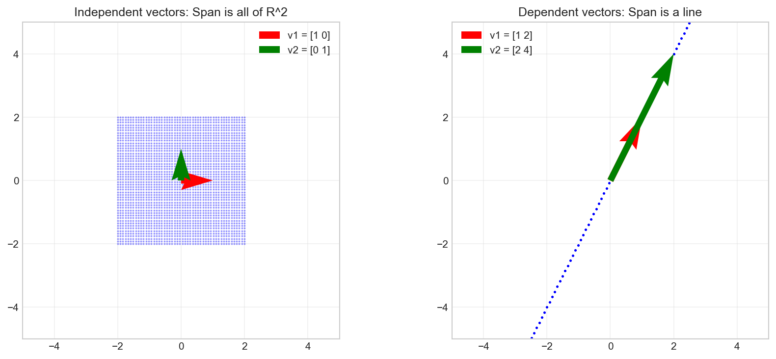
Span
The span of a set of vectors is the set of all possible linear combinations of those vectors:
# Visualize the span of two vectors in R^2
def plot_span_2d(v1, v2, ax, title):
    """Visualize the span of two 2D vectors."""
    # Generate random linear combinations
    t = np.linspace(-2, 2, 50)
    s = np.linspace(-2, 2, 50)
    T, S = np.meshgrid(t, s)

    # Points in the span
    X = T * v1[0] + S * v2[0]
    Y = T * v1[1] + S * v2[1]

    ax.scatter(X.flatten(), Y.flatten(), alpha=0.3, s=1, c='blue')
    ax.quiver(0, 0, v1[0], v1[1], angles='xy', scale_units='xy', scale=1,
              color='red', width=0.02, label=f'v1 = {v1}')
    ax.quiver(0, 0, v2[0], v2[1], angles='xy', scale_units='xy', scale=1,
              color='green', width=0.02, label=f'v2 = {v2}')
    ax.set_xlim(-5, 5)
    ax.set_ylim(-5, 5)
    ax.set_aspect('equal')
    ax.grid(True, alpha=0.3)
    ax.legend()
    ax.set_title(title)

fig, axes = plt.subplots(1, 2, figsize=(12, 5))

# Two independent vectors span R^2
plot_span_2d(np.array([1, 0]), np.array([0, 1]), axes[0],
             'Independent vectors: Span is all of R^2')

# Two dependent vectors span a line
plot_span_2d(np.array([1, 2]), np.array([2, 4]), axes[1],
             'Dependent vectors: Span is a line')

plt.tight_layout()
plt.show()
Basis
A basis for a vector space $V$ is a set of vectors that:
- Are linearly independent
- Span $V$
The dimension of a vector space is the number of vectors in any basis.
# Standard basis for R^3
e1 = np.array([1, 0, 0])
e2 = np.array([0, 1, 0])
e3 = np.array([0, 0, 1])

print("Standard basis for R^3:")
print(f"e1 = {e1}")
print(f"e2 = {e2}")
print(f"e3 = {e3}")

# Any vector in R^3 can be written as a linear combination
v = np.array([3, -2, 5])
print(f"\nVector v = {v}")
print(f"v = {v[0]}*e1 + {v[1]}*e2 + {v[2]}*e3")
print(f"Verification: {v[0]*e1 + v[1]*e2 + v[2]*e3}")
Standard basis for R^3:
e1 = [1 0 0]
e2 = [0 1 0]
e3 = [0 0 1]

Vector v = [ 3 -2  5]
v = 3*e1 + -2*e2 + 5*e3
Verification: [ 3 -2  5]
Non-Standard Bases
Any set of linearly independent vectors that span the space can serve as a basis:
# Alternative basis for R^2
b1 = np.array([1, 1])
b2 = np.array([1, -1])

# Check it's a valid basis
independent, rank = check_linear_independence([b1, b2])
print(f"b1 = {b1}, b2 = {b2}")
print(f"Linearly independent: {independent}")
print(f"Spans R^2: {rank == 2}\n")

# Express a vector in this basis
v = np.array([3, 1])
# v = c1*b1 + c2*b2
# Solve for coefficients
B = np.column_stack([b1, b2])
coeffs = np.linalg.solve(B, v)
print(f"Vector v = {v} in standard basis")
print(f"v = {coeffs[0]}*b1 + {coeffs[1]}*b2 in new basis")
print(f"Coefficients in new basis: {coeffs}")
b1 = [1 1], b2 = [ 1 -1]
Linearly independent: True
Spans R^2: True

Vector v = [3 1] in standard basis
v = 2.0*b1 + 1.0*b2 in new basis
Coefficients in new basis: [2. 1.]
Subspaces
A subspace of a vector space $V$ is a subset $W \subseteq V$ that is itself a vector space under the same operations. To verify $W$ is a subspace:
- The zero vector is in $W$
- $W$ is closed under addition
- $W$ is closed under scalar multiplication
Column Space (Range)
The column space (or range) of a matrix $\boldsymbol{A}$ is the span of its columns:
It represents all possible outputs of the linear transformation defined by $\boldsymbol{A}$.
# Find a basis for the column space
A = np.array([[1, 2, 3],
              [4, 5, 6],
              [7, 8, 9]])

print(f"Matrix A:\n{A}\n")
print(f"Rank of A: {np.linalg.matrix_rank(A)}")

# The rank tells us the dimension of the column space
# Use SVD to find an orthonormal basis for the column space
U, s, Vt = np.linalg.svd(A)

# The first r columns of U form an orthonormal basis for Col(A)
r = np.linalg.matrix_rank(A)
col_space_basis = U[:, :r]
print(f"\nOrthonormal basis for column space (first {r} columns of U):")
print(col_space_basis)
Matrix A:
[[1 2 3]
 [4 5 6]
 [7 8 9]]

Rank of A: 2

Orthonormal basis for column space (first 2 columns of U):
[[-0.21483724  0.88723069]
 [-0.52058739  0.24964395]
 [-0.82633754 -0.38794278]]
Null Space (Kernel)
The null space (or kernel) of a matrix $\boldsymbol{A}$ is the set of all vectors that map to zero:
from scipy.linalg import null_space

# Find the null space of A
null_A = null_space(A)
print(f"Null space of A (basis vectors):\n{null_A}\n")

# Verify: A @ null_vector should be approximately zero
if null_A.size > 0:
    result = A @ null_A
    print(f"A @ null_space_basis =\n{result}")
    print(f"All entries near zero: {np.allclose(result, 0)}")
Null space of A (basis vectors):
[[ 0.40824829]
 [-0.81649658]
 [ 0.40824829]]

A @ null_space_basis =
[[-4.44089210e-16]
 [-8.88178420e-16]
 [-1.33226763e-15]]
All entries near zero: True
The Fundamental Theorem of Linear Algebra
For an $m \times n$ matrix $\boldsymbol{A}$ with rank $r$:
- $\dim(\text{Col}(\boldsymbol{A})) = r$ (column space dimension)
- $\dim(\text{Null}(\boldsymbol{A})) = n - r$ (null space dimension)
- $\dim(\text{Row}(\boldsymbol{A})) = r$ (row space dimension)
- $\dim(\text{Null}(\boldsymbol{A}^T)) = m - r$ (left null space dimension)
def analyze_matrix_spaces(A):
    """Analyze the four fundamental subspaces of a matrix."""
    m, n = A.shape
    r = np.linalg.matrix_rank(A)

    print(f"Matrix dimensions: {m} x {n}")
    print(f"Rank: {r}\n")

    print("Fundamental Subspaces:")
    print(f"  Column space:    dimension = {r} (subspace of R^{m})")
    print(f"  Null space:      dimension = {n - r} (subspace of R^{n})")
    print(f"  Row space:       dimension = {r} (subspace of R^{n})")
    print(f"  Left null space: dimension = {m - r} (subspace of R^{m})")

# Example
B = np.array([[1, 2, 3, 4],
              [2, 4, 6, 8],
              [1, 1, 1, 1]])

print(f"Matrix B:\n{B}\n")
analyze_matrix_spaces(B)
Matrix B:
[[1 2 3 4]
 [2 4 6 8]
 [1 1 1 1]]

Matrix dimensions: 3 x 4
Rank: 2

Fundamental Subspaces:
  Column space:    dimension = 2 (subspace of R^3)
  Null space:      dimension = 2 (subspace of R^4)
  Row space:       dimension = 2 (subspace of R^4)
  Left null space: dimension = 1 (subspace of R^3)
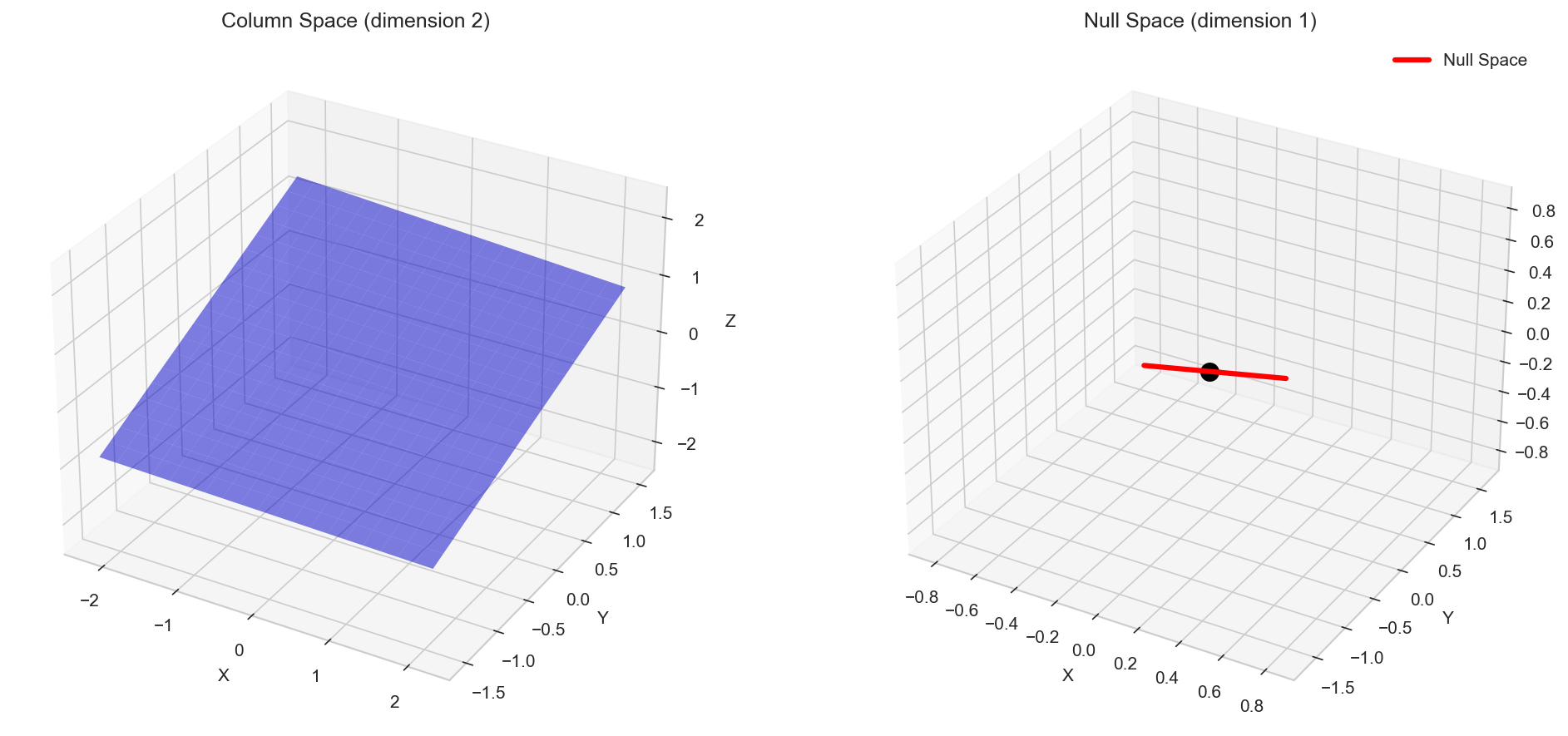
Visualizing Subspaces in 3D
Let’s visualize the column space and null space for a 3x3 rank-2 matrix:
# Create a rank-2 matrix in R^3
C = np.array([[1, 2, 3],
              [4, 5, 6],
              [7, 8, 9]])

# Get column space basis
U, s, Vt = np.linalg.svd(C)
r = np.linalg.matrix_rank(C)
col_basis = U[:, :r]

# Get null space
null_basis = null_space(C)

fig = plt.figure(figsize=(12, 5))

# Plot column space (a plane through origin)
ax1 = fig.add_subplot(121, projection='3d')
t = np.linspace(-2, 2, 20)
T, S = np.meshgrid(t, t)
X = T * col_basis[0, 0] + S * col_basis[0, 1]
Y = T * col_basis[1, 0] + S * col_basis[1, 1]
Z = T * col_basis[2, 0] + S * col_basis[2, 1]
ax1.plot_surface(X, Y, Z, alpha=0.5, color='blue')
ax1.set_xlabel('X')
ax1.set_ylabel('Y')
ax1.set_zlabel('Z')
ax1.set_title(f'Column Space (dimension {r})')

# Plot null space (a line through origin)
ax2 = fig.add_subplot(122, projection='3d')
t = np.linspace(-2, 2, 100)
null_vec = null_basis.flatten()
ax2.plot(t * null_vec[0], t * null_vec[1], t * null_vec[2],
         'r-', linewidth=3, label='Null Space')
ax2.scatter([0], [0], [0], color='black', s=100)
ax2.set_xlabel('X')
ax2.set_ylabel('Y')
ax2.set_zlabel('Z')
ax2.set_title(f'Null Space (dimension {3-r})')
ax2.legend()

plt.tight_layout()
plt.show()
Orthogonal Complements
Two subspaces are orthogonal complements if every vector in one is perpendicular to every vector in the other, and together they span the entire space.
- The null space is the orthogonal complement of the row space
- The left null space is the orthogonal complement of the column space
# Verify orthogonality between row space and null space
row_space_basis = Vt[:r, :].T  # First r rows of Vt, transposed to columns
null_space_vector = null_basis.flatten()

# Dot product should be zero
for i in range(r):
    dot_product = np.dot(row_space_basis[:, i], null_space_vector)
    print(f"Row space basis vector {i+1} dot null space: {dot_product:.10f}")
Row space basis vector 1 dot null space: -0.0000000000
Row space basis vector 2 dot null space: 0.0000000000
Summary
In this article, we covered:
- Vector spaces: Sets closed under addition and scalar multiplication
- Linear independence: Vectors with no redundant information
- Span: All possible linear combinations of vectors
- Basis and dimension: Minimal spanning sets
- Subspaces: Vector spaces within vector spaces
- Column space: The range of a matrix transformation
- Null space: Vectors that map to zero
- Fundamental theorem: The relationship between the four fundamental subspaces
Understanding these concepts is essential for eigenvalue analysis, which we’ll explore in the next article.
Resources
Linear Algebra: Python Series - View all articles in this series.
This blog post, titled: "Linear Algebra: Vector Spaces and Subspaces: Linear Algebra Crash Course for Programmers Part 5" by Craig Johnston, is licensed under a Creative Commons Attribution 4.0 International License.
