This article on systems of linear equations is part three of an ongoing crash course on programming with linear algebra, demonstrating concepts and implementations in Python. We’ll explore how matrices provide a powerful framework for solving systems of equations, a fundamental problem that appears throughout science, engineering, and machine learning.
Linear Algebra: Python Series - View all articles in this series.
Previous articles in this series:
This series began with Linear Algebra: Vectors Crash Course for Python Programmers Part 1 and continued with Linear Algebra: Matrices 1. Understanding matrix operations from those articles is essential for this topic.
This small series of articles on linear algebra is meant to help in preparation for learning the more profound concepts related to Machine Learning, AI, and the math that drives the higher level abstractions provided by many of the libraries available today.
Python examples in this article make use of the Numpy library. Read the article Python Data Essentials - Numpy if you want a quick overview of this important Python library along with the Matplotlib Python library for visualizations.
import numpy as np
import matplotlib.pyplot as plt

%matplotlib inline
What is a System of Linear Equations?
A system of linear equations is a collection of linear equations involving the same set of variables. The goal is to find values for the variables that satisfy all equations simultaneously.
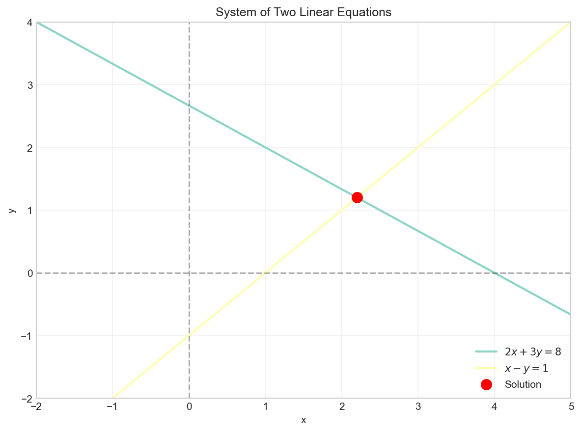
Consider a simple example with two equations and two unknowns:
Geometrically, each linear equation in two variables represents a line. The solution to the system is the point where the lines intersect.
# Visualize the system of equations
x = np.linspace(-2, 5, 100)

# 2x + 3y = 8  =>  y = (8 - 2x) / 3
y1 = (8 - 2*x) / 3

# x - y = 1  =>  y = x - 1
y2 = x - 1

plt.figure(figsize=(8, 6))
plt.plot(x, y1, label='$2x + 3y = 8$', linewidth=2)
plt.plot(x, y2, label='$x - y = 1$', linewidth=2)
plt.scatter([2.2], [1.2], color='red', s=100, zorder=5, label='Solution')
plt.axhline(y=0, color='k', linestyle='--', alpha=0.3)
plt.axvline(x=0, color='k', linestyle='--', alpha=0.3)
plt.grid(True, alpha=0.3)
plt.xlabel('x')
plt.ylabel('y')
plt.legend()
plt.title('System of Two Linear Equations')
plt.axis((-2, 5, -2, 4))
plt.show()
Matrix Representation
Any system of linear equations can be written in matrix form as:
Where:
- $\boldsymbol{A}$ is the coefficient matrix
- $\vec{x}$ is the variable vector (unknowns)
- $\vec{b}$ is the constant vector
For this example:
# Define the coefficient matrix A and constant vector b
A = np.array([[2, 3],
              [1, -1]])

b = np.array([8, 1])

print(f"Coefficient matrix A:\n{A}\n")
print(f"Constant vector b:\n{b}")
Coefficient matrix A:
[[ 2  3]
 [ 1 -1]]

Constant vector b:
[8 1]
Solving Systems with NumPy
NumPy provides the np.linalg.solve() function to solve systems of linear equations. This function uses optimized algorithms (typically LU decomposition) to find the solution efficiently.
# Solve the system Ax = b
x = np.linalg.solve(A, b)
print(f"Solution: x = {x[0]:.4f}, y = {x[1]:.4f}")
Solution: x = 2.2000, y = 1.2000
# Verify the solution
result = A @ x
print(f"A @ x = {result}")
print(f"b     = {b}")
print(f"Match: {np.allclose(result, b)}")
A @ x = [8. 1.]
b     = [8 1]
Match: True
Augmented Matrices
An augmented matrix combines the coefficient matrix $\boldsymbol{A}$ and the constant vector $\vec{b}$ into a single matrix. This representation is useful for manual row reduction techniques.
# Create an augmented matrix
augmented = np.column_stack((A, b))
print(f"Augmented matrix:\n{augmented}")
Augmented matrix:
[[ 2  3  8]
 [ 1 -1  1]]
Gaussian Elimination
Gaussian elimination (or row reduction) is a systematic method for solving systems of linear equations. The process transforms the augmented matrix into row echelon form (REF) or reduced row echelon form (RREF).
Row Operations
Three elementary row operations are allowed:
- Swap two rows
- Multiply a row by a nonzero scalar
- Add a multiple of one row to another row
Example: Step-by-Step Row Reduction
Let’s solve a larger system:
# Define the system
A_large = np.array([[1, 2, 1],
                    [2, -1, 3],
                    [3, 1, -1]], dtype=float)

b_large = np.array([9, 8, 3], dtype=float)

# Create augmented matrix
aug = np.column_stack((A_large, b_large))
print(f"Initial augmented matrix:\n{aug}\n")
Initial augmented matrix:
[[ 1.  2.  1.  9.]
 [ 2. -1.  3.  8.]
 [ 3.  1. -1.  3.]]
# Step 1: Eliminate x from row 2 (R2 = R2 - 2*R1)
aug[1] = aug[1] - 2 * aug[0]
print(f"After R2 = R2 - 2*R1:\n{aug}\n")

# Step 2: Eliminate x from row 3 (R3 = R3 - 3*R1)
aug[2] = aug[2] - 3 * aug[0]
print(f"After R3 = R3 - 3*R1:\n{aug}\n")

# Step 3: Make pivot in row 2 equal to 1 (R2 = R2 / -5)
aug[1] = aug[1] / -5
print(f"After R2 = R2 / -5:\n{aug}\n")

# Step 4: Eliminate y from row 3 (R3 = R3 + 5*R2)
aug[2] = aug[2] + 5 * aug[1]
print(f"After R3 = R3 + 5*R2:\n{aug}\n")

# Step 5: Make pivot in row 3 equal to 1 (R3 = R3 / -6)
aug[2] = aug[2] / -6
print(f"After R3 = R3 / -6:\n{aug}")
After R2 = R2 - 2*R1:
[[  1.   2.   1.   9.]
 [  0.  -5.   1. -10.]
 [  3.   1.  -1.   3.]]

After R3 = R3 - 3*R1:
[[  1.   2.   1.   9.]
 [  0.  -5.   1. -10.]
 [  0.  -5.  -4. -24.]]

After R2 = R2 / -5:
[[ 1.   2.   1.   9. ]
 [-0.   1.  -0.2  2. ]
 [ 0.  -5.  -4. -24. ]]

After R3 = R3 + 5*R2:
[[  1.    2.    1.    9. ]
 [ -0.    1.   -0.2   2. ]
 [  0.    0.   -5.  -14. ]]

After R3 = R3 / -6:
[[ 1.          2.          1.          9.        ]
 [-0.          1.         -0.2         2.        ]
 [-0.         -0.          1.          2.8       ]]
Now we have the matrix in row echelon form. We can use back substitution to find the solution:
# Back substitution
z = aug[2, 3]
y = aug[1, 3] - aug[1, 2] * z
x = aug[0, 3] - aug[0, 1] * y - aug[0, 2] * z

print(f"Solution: x = {x:.4f}, y = {y:.4f}, z = {z:.4f}")
Solution: x = 1.6000, y = 2.5600, z = 2.8000
# Verify with np.linalg.solve
solution = np.linalg.solve(A_large, b_large)
print(f"NumPy solution: {solution}")
NumPy solution: [1.6 2.56 2.8 ]
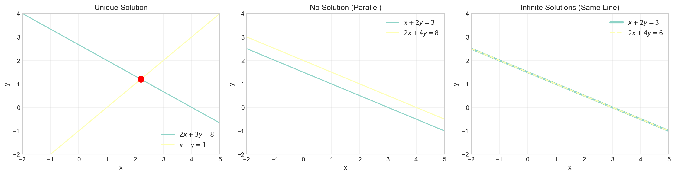
Types of Solutions
A system of linear equations can have:
- Exactly one solution (consistent, independent): Lines intersect at one point
- No solution (inconsistent): Lines are parallel
- Infinitely many solutions (consistent, dependent): Lines are the same
Determining Solution Type
The rank of a matrix helps determine the type of solution:
- If $rank(\boldsymbol{A}) = rank([\boldsymbol{A}|\vec{b}]) = n$ (number of variables): unique solution
- If $rank(\boldsymbol{A}) < rank([\boldsymbol{A}|\vec{b}])$: no solution
- If $rank(\boldsymbol{A}) = rank([\boldsymbol{A}|\vec{b}]) < n$: infinitely many solutions
# Example 1: Unique solution (already shown above)
A1 = np.array([[2, 3], [1, -1]])
b1 = np.array([8, 1])
print(f"Example 1 - Unique solution:")
print(f"  rank(A) = {np.linalg.matrix_rank(A1)}")
print(f"  rank([A|b]) = {np.linalg.matrix_rank(np.column_stack((A1, b1)))}")
print(f"  Solution: {np.linalg.solve(A1, b1)}\n")
Example 1 - Unique solution:
  rank(A) = 2
  rank([A|b]) = 2
  Solution: [2.2 1.2]
# Example 2: No solution (parallel lines)
A2 = np.array([[1, 2], [2, 4]])
b2 = np.array([3, 8])  # 2*(first equation) would give y=6, not 8
print(f"Example 2 - No solution (parallel lines):")
print(f"  rank(A) = {np.linalg.matrix_rank(A2)}")
print(f"  rank([A|b]) = {np.linalg.matrix_rank(np.column_stack((A2, b2)))}")
print(f"  rank(A) < rank([A|b]), so no solution exists\n")
Example 2 - No solution (parallel lines):
  rank(A) = 1
  rank([A|b]) = 2
  rank(A) < rank([A|b]), so no solution exists
# Example 3: Infinitely many solutions (same line)
A3 = np.array([[1, 2], [2, 4]])
b3 = np.array([3, 6])  # Second equation is 2*(first equation)
print(f"Example 3 - Infinitely many solutions:")
print(f"  rank(A) = {np.linalg.matrix_rank(A3)}")
print(f"  rank([A|b]) = {np.linalg.matrix_rank(np.column_stack((A3, b3)))}")
print(f"  rank(A) = rank([A|b]) < n, so infinitely many solutions")
Example 3 - Infinitely many solutions:
  rank(A) = 1
  rank([A|b]) = 1
  rank(A) = rank([A|b]) < n, so infinitely many solutions
Visualizing Solution Types
fig, axes = plt.subplots(1, 3, figsize=(15, 4))
x = np.linspace(-2, 5, 100)

# Plot 1: Unique solution
ax1 = axes[0]
ax1.plot(x, (8 - 2*x)/3, label='$2x + 3y = 8$')
ax1.plot(x, x - 1, label='$x - y = 1$')
ax1.scatter([2.2], [1.2], color='red', s=100, zorder=5)
ax1.set_title('Unique Solution')
ax1.set_xlabel('x')
ax1.set_ylabel('y')
ax1.legend()
ax1.grid(True, alpha=0.3)
ax1.set_xlim(-2, 5)
ax1.set_ylim(-2, 4)

# Plot 2: No solution (parallel lines)
ax2 = axes[1]
ax2.plot(x, (3 - x)/2, label='$x + 2y = 3$')
ax2.plot(x, (8 - 2*x)/4, label='$2x + 4y = 8$')
ax2.set_title('No Solution (Parallel)')
ax2.set_xlabel('x')
ax2.set_ylabel('y')
ax2.legend()
ax2.grid(True, alpha=0.3)
ax2.set_xlim(-2, 5)
ax2.set_ylim(-2, 4)

# Plot 3: Infinite solutions (same line)
ax3 = axes[2]
ax3.plot(x, (3 - x)/2, label='$x + 2y = 3$', linewidth=3)
ax3.plot(x, (6 - 2*x)/4, label='$2x + 4y = 6$', linestyle='--', linewidth=2)
ax3.set_title('Infinite Solutions (Same Line)')
ax3.set_xlabel('x')
ax3.set_ylabel('y')
ax3.legend()
ax3.grid(True, alpha=0.3)
ax3.set_xlim(-2, 5)
ax3.set_ylim(-2, 4)

plt.tight_layout()
plt.show()
Practical Application: Network Flow
Systems of linear equations appear in many real-world applications. Consider a simple network flow problem where we need to determine flow rates through a network.
# Network flow example: Water distribution
# Node balance equations (flow in = flow out)
#
#       x1          x2
#   [1]---->[2]---->[4]
#    |       |       |
#    |x4     |x3     |x5
#    v       v       v
#   [3]---->[5]---->[6]
#       x6      x7
#
# Given: Total inflow at [1] = 100, outflow at [4] = 40, outflow at [6] = 60
# Constraint equations from node balance:

A_flow = np.array([
    [1, 0, 0, 1, 0, 0, 0],    # Node 1: x1 + x4 = 100
    [1, -1, -1, 0, 0, 0, 0],   # Node 2: x1 = x2 + x3
    [0, 0, 0, 1, 0, -1, 0],    # Node 3: x4 = x6
    [0, 1, 0, 0, 1, 0, 0],     # Node 4: x2 + x5 = 40
    [0, 0, 1, 0, 0, 1, -1],    # Node 5: x3 + x6 = x7
    [0, 0, 0, 0, 1, 0, 1],     # Node 6: x5 + x7 = 60
    [0, 0, 1, 0, -1, 0, 0]     # Additional constraint: x3 = x5
])

b_flow = np.array([100, 0, 0, 40, 0, 60, 0])

# Solve
flow_solution = np.linalg.solve(A_flow, b_flow)
print("Network flow solution:")
for i, val in enumerate(flow_solution, 1):
    print(f"  x{i} = {val:.2f}")
Network flow solution:
  x1 = 60.00
  x2 = 20.00
  x3 = 40.00
  x4 = 40.00
  x5 = 20.00
  x6 = 40.00
  x7 = 40.00
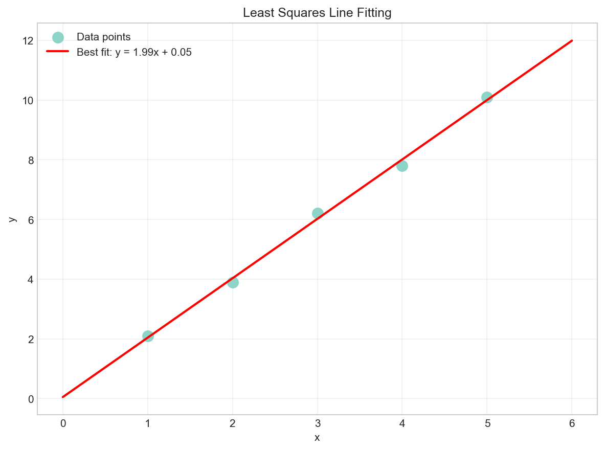
Least Squares for Overdetermined Systems
When a system has more equations than unknowns (overdetermined), there may be no exact solution. In such cases, we can find the least squares solution that minimizes the error.
The least squares solution is given by the normal equations:
# Overdetermined system: fit a line to 5 points
# y = mx + c
points = np.array([[1, 2.1], [2, 3.9], [3, 6.2], [4, 7.8], [5, 10.1]])

# Set up Ax = b where A = [[x, 1], ...] and b = [y, ...]
A_ls = np.column_stack((points[:, 0], np.ones(len(points))))
b_ls = points[:, 1]

print(f"Coefficient matrix A (overdetermined):\n{A_ls}\n")
print(f"Constant vector b:\n{b_ls}\n")

# Solve using least squares
solution_ls, residuals, rank, s = np.linalg.lstsq(A_ls, b_ls, rcond=None)
print(f"Least squares solution: m = {solution_ls[0]:.4f}, c = {solution_ls[1]:.4f}")
Coefficient matrix A (overdetermined):
[[1. 1.]
 [2. 1.]
 [3. 1.]
 [4. 1.]
 [5. 1.]]

Constant vector b:
[ 2.1  3.9  6.2  7.8 10.1]

Least squares solution: m = 1.9900, c = 0.0600
# Visualize the least squares fit
plt.figure(figsize=(8, 6))
plt.scatter(points[:, 0], points[:, 1], s=100, label='Data points')
x_line = np.linspace(0, 6, 100)
y_line = solution_ls[0] * x_line + solution_ls[1]
plt.plot(x_line, y_line, 'r-', linewidth=2,
         label=f'Best fit: y = {solution_ls[0]:.2f}x + {solution_ls[1]:.2f}')
plt.xlabel('x')
plt.ylabel('y')
plt.legend()
plt.title('Least Squares Line Fitting')
plt.grid(True, alpha=0.3)
plt.show()
Summary
In this article, we covered:
- Matrix representation of systems of linear equations: $\boldsymbol{A}\vec{x} = \vec{b}$
- Gaussian elimination for solving systems step by step
- NumPy’s
np.linalg.solve()for efficient solutions - Types of solutions: unique, none, or infinitely many
- Using matrix rank to determine solution type
- Least squares for overdetermined systems
In the next article, we’ll explore matrix inverses and determinants, which provide another approach to solving systems and reveal important properties of matrices.
Resources
- Systems of Linear Equations - Khan Academy
- Gaussian Elimination - Wikipedia
- NumPy Linear Algebra Documentation
- Least Squares - Wikipedia
Linear Algebra: Python Series - View all articles in this series.
This blog post, titled: "Linear Algebra: Systems of Linear Equations: Linear Algebra Crash Course for Programmers Part 3" by Craig Johnston, is licensed under a Creative Commons Attribution 4.0 International License.
