This article continues the exploration of eigenvalues and eigenvectors, focusing on diagonalization, computing matrix powers, and handling complex eigenvalues. Part seven of the series.
Linear Algebra: Python Series - View all articles in this series.
Previous articles in this series:
- Linear Algebra: Vectors
- Linear Algebra: Matrices
- Linear Algebra: Systems of Linear Equations
- Linear Algebra: Matrix Inverses and Determinants
- Linear Algebra: Vector Spaces and Subspaces
- Linear Algebra: Eigenvalues and Eigenvectors Part 1
See Part 1 for the fundamentals of eigenvalues and eigenvectors.
Python examples use NumPy and Matplotlib.
import numpy as np
import matplotlib.pyplot as plt

%matplotlib inline
Diagonalization
A matrix $\boldsymbol{A}$ is diagonalizable if it can be written as:
Where:
- $\boldsymbol{D}$ is a diagonal matrix containing the eigenvalues
- $\boldsymbol{P}$ is a matrix whose columns are the corresponding eigenvectors
# Create a diagonalizable matrix
A = np.array([[4, 1],
              [2, 3]])

# Get eigenvalues and eigenvectors
eigenvalues, P = np.linalg.eig(A)

print(f"Matrix A:\n{A}\n")
print(f"Eigenvalues: {eigenvalues}")
print(f"\nEigenvector matrix P:\n{P}")
Matrix A:
[[4 1]
 [2 3]]

Eigenvalues: [5. 2.]

Eigenvector matrix P:
[[ 0.70710678 -0.4472136 ]
 [ 0.70710678  0.89442719]]
# Construct the diagonal matrix D
D = np.diag(eigenvalues)
print(f"Diagonal matrix D:\n{D}")
Diagonal matrix D:
[[5. 0.]
 [0. 2.]]
# Verify: A = P @ D @ P^(-1)
P_inv = np.linalg.inv(P)
reconstructed = P @ D @ P_inv

print(f"P @ D @ P^(-1):\n{reconstructed}")
print(f"\nEquals A: {np.allclose(A, reconstructed)}")
P @ D @ P^(-1):
[[4. 1.]
 [2. 3.]]

Equals A: True
Computing Matrix Powers Efficiently
One of the key applications of diagonalization is efficiently computing matrix powers. Since:
And $\boldsymbol{D}^n$ is simply the diagonal matrix with $\lambda_i^n$ on the diagonal.
def matrix_power_via_diagonalization(A, n):
    """Compute A^n using diagonalization."""
    eigenvalues, P = np.linalg.eig(A)
    D_n = np.diag(eigenvalues ** n)
    P_inv = np.linalg.inv(P)
    return P @ D_n @ P_inv

# Compute A^10
n = 10
A_n_diag = matrix_power_via_diagonalization(A, n)
A_n_direct = np.linalg.matrix_power(A, n)

print(f"A^{n} via diagonalization:\n{A_n_diag}\n")
print(f"A^{n} via direct computation:\n{A_n_direct}\n")
print(f"Results match: {np.allclose(A_n_diag, A_n_direct)}")
A^10 via diagonalization:
[[6510418. 1627603.]
 [3255206. 3255215.]]

A^10 via direct computation:
[[6510418 1627603]
 [3255206 3255215]]

Results match: True
Application: Fibonacci Numbers
The Fibonacci sequence can be computed using matrix powers:
def fibonacci_matrix(n):
    """Compute nth Fibonacci number using matrix power."""
    F = np.array([[1, 1],
                  [1, 0]], dtype=np.float64)
    if n == 0:
        return 0
    result = np.linalg.matrix_power(F, n)
    return int(round(result[0, 1]))

# Compute Fibonacci numbers
print("Fibonacci sequence (first 15 numbers):")
for i in range(15):
    print(f"F({i}) = {fibonacci_matrix(i)}")
Fibonacci sequence (first 15 numbers):
F(0) = 0
F(1) = 1
F(2) = 1
F(3) = 2
F(4) = 3
F(5) = 5
F(6) = 8
F(7) = 13
F(8) = 21
F(9) = 34
F(10) = 55
F(11) = 89
F(12) = 144
F(13) = 233
F(14) = 377
Complex Eigenvalues
Some matrices have complex eigenvalues, particularly rotation matrices:
# 90-degree rotation matrix
theta = np.pi / 2
R = np.array([[np.cos(theta), -np.sin(theta)],
              [np.sin(theta),  np.cos(theta)]])

eigenvalues_R, eigenvectors_R = np.linalg.eig(R)

print(f"90-degree rotation matrix:\n{R}\n")
print(f"Eigenvalues: {eigenvalues_R}")
print(f"\nNote: These are complex numbers (i = sqrt(-1))")
90-degree rotation matrix:
[[ 6.123234e-17 -1.000000e+00]
 [ 1.000000e+00  6.123234e-17]]

Eigenvalues: [6.12323400e-17+1.j 6.12323400e-17-1.j]

Note: These are complex numbers (i = sqrt(-1))
Complex eigenvalues always come in conjugate pairs for real matrices:
# A matrix with complex eigenvalues
B = np.array([[1, -2],
              [1,  1]])

eigenvalues_B, eigenvectors_B = np.linalg.eig(B)

print(f"Matrix B:\n{B}\n")
print(f"Eigenvalues: {eigenvalues_B}")
print(f"\nReal part: {eigenvalues_B.real}")
print(f"Imaginary part: {eigenvalues_B.imag}")
Matrix B:
[[ 1 -2]
 [ 1  1]]

Eigenvalues: [1.+1.41421356j 1.-1.41421356j]

Real part: [1. 1.]
Imaginary part: [ 1.41421356 -1.41421356]
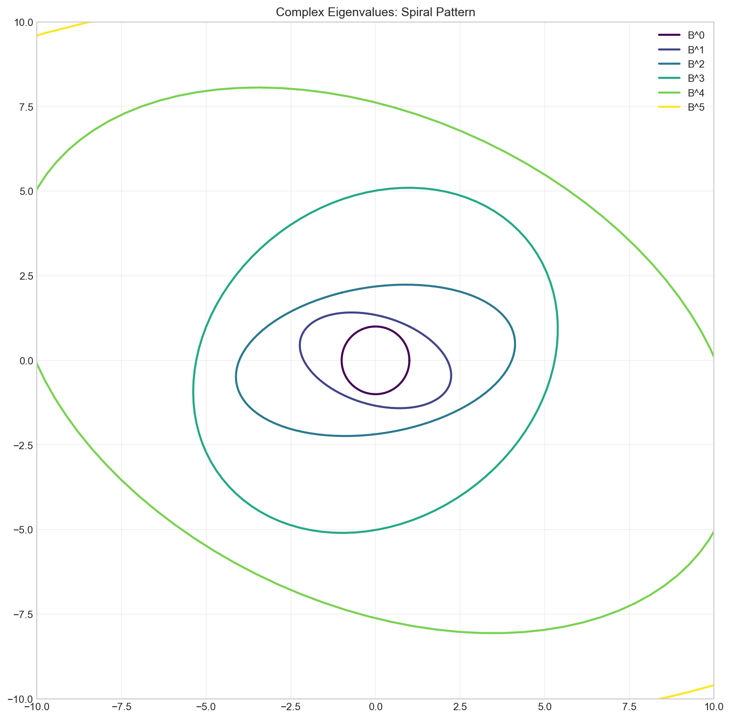
Geometric Meaning of Complex Eigenvalues
Complex eigenvalues indicate rotation combined with scaling:
- The magnitude $|\lambda| = \sqrt{a^2 + b^2}$ is the scaling factor
- The argument $\theta = \arctan(b/a)$ is the rotation angle
# Visualize the transformation
fig, ax = plt.subplots(figsize=(8, 8))

# Original vectors
t = np.linspace(0, 2*np.pi, 100)
circle = np.vstack([np.cos(t), np.sin(t)])

# Apply transformation multiple times
colors = plt.cm.viridis(np.linspace(0, 1, 6))
current = circle.copy()

for i in range(6):
    ax.plot(current[0], current[1], color=colors[i],
            linewidth=2, label=f'B^{i}')
    current = B @ current

ax.set_xlim(-10, 10)
ax.set_ylim(-10, 10)
ax.set_aspect('equal')
ax.grid(True, alpha=0.3)
ax.legend()
ax.set_title('Repeated application of B: Spiral pattern')
plt.show()

# Compute magnitude and angle
lambda1 = eigenvalues_B[0]
magnitude = np.abs(lambda1)
angle = np.angle(lambda1) * 180 / np.pi

print(f"Scaling factor: {magnitude:.4f}")
print(f"Rotation angle: {angle:.2f} degrees")
When is a Matrix Not Diagonalizable?
A matrix may not be diagonalizable if it has repeated eigenvalues with insufficient eigenvectors:
# A non-diagonalizable matrix
C = np.array([[2, 1],
              [0, 2]])

eigenvalues_C, eigenvectors_C = np.linalg.eig(C)

print(f"Matrix C:\n{C}\n")
print(f"Eigenvalues: {eigenvalues_C}")
print(f"\nEigenvectors:\n{eigenvectors_C}")
print(f"\nNote: Eigenvalue 2 has multiplicity 2, but only one eigenvector.")
Matrix C:
[[2 1]
 [0 2]]

Eigenvalues: [2. 2.]

Eigenvectors:
[[1.         1.        ]
 [0.         0.00000001]]

Note: Eigenvalue 2 has multiplicity 2, but only one eigenvector.
# Check if P is invertible
det_P = np.linalg.det(eigenvectors_C)
print(f"Determinant of eigenvector matrix: {det_P}")
print(f"Matrix is {'diagonalizable' if not np.isclose(det_P, 0) else 'NOT diagonalizable'}")
Determinant of eigenvector matrix: 1.0000000149011612e-08
Matrix is NOT diagonalizable
The Matrix Exponential
The matrix exponential $e^{\boldsymbol{A}}$ is defined using the power series:
For diagonalizable matrices:
from scipy.linalg import expm

# Matrix exponential
A = np.array([[1, 2],
              [0, 3]])

exp_A = expm(A)
print(f"Matrix A:\n{A}\n")
print(f"e^A:\n{exp_A}")
Matrix A:
[[1 2]
 [0 3]]

e^A:
[[ 2.71828183 17.3673271 ]
 [ 0.         20.08553692]]
# Via diagonalization
eigenvalues_A, P = np.linalg.eig(A)
exp_D = np.diag(np.exp(eigenvalues_A))
P_inv = np.linalg.inv(P)

exp_A_diag = P @ exp_D @ P_inv
print(f"e^A via diagonalization:\n{exp_A_diag}")
print(f"\nResults match: {np.allclose(exp_A, exp_A_diag)}")
e^A via diagonalization:
[[ 2.71828183 17.3673271 ]
 [ 0.         20.08553692]]

Results match: True
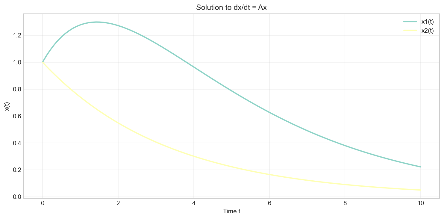
Application: Solving Differential Equations
The system of differential equations:
has solution:
# Solve dx/dt = Ax
A = np.array([[-0.5, 1],
              [0, -0.3]])

x0 = np.array([1, 1])

# Compute solution at different times
t_values = np.linspace(0, 10, 100)
solutions = []

for t in t_values:
    x_t = expm(A * t) @ x0
    solutions.append(x_t)

solutions = np.array(solutions)

plt.figure(figsize=(10, 5))
plt.plot(t_values, solutions[:, 0], label='x1(t)')
plt.plot(t_values, solutions[:, 1], label='x2(t)')
plt.xlabel('Time t')
plt.ylabel('x(t)')
plt.title('Solution to dx/dt = Ax')
plt.legend()
plt.grid(True, alpha=0.3)
plt.show()
Summary
In this article, we covered:
- Diagonalization: $\boldsymbol{A} = \boldsymbol{P}\boldsymbol{D}\boldsymbol{P}^{-1}$
- Efficient matrix powers using diagonalization
- Fibonacci numbers via matrix exponentiation
- Complex eigenvalues: rotation and scaling
- Non-diagonalizable matrices: deficient eigenvectors
- Matrix exponential and differential equations
Resources
Linear Algebra: Python Series - View all articles in this series.
This blog post, titled: "Linear Algebra: Eigenvalues and Eigenvectors Part 2: Linear Algebra Crash Course for Programmers Part 7" by Craig Johnston, is licensed under a Creative Commons Attribution 4.0 International License.
