This article on eigenvalues and eigenvectors is part six of an ongoing crash course on programming with linear algebra. Eigenvalues and eigenvectors are among the most important concepts in linear algebra, with applications ranging from differential equations to machine learning algorithms like PCA.
Linear Algebra: Python Series - View all articles in this series.
Previous articles in this series:
- Linear Algebra: Vectors
- Linear Algebra: Matrices
- Linear Algebra: Systems of Linear Equations
- Linear Algebra: Matrix Inverses and Determinants
- Linear Algebra: Vector Spaces and Subspaces
Previous articles covered Vectors, Matrices, Systems of Equations, Inverses and Determinants, and Vector Spaces.
Python examples in this article make use of the Numpy library.
import numpy as np
import matplotlib.pyplot as plt

%matplotlib inline
What are Eigenvectors and Eigenvalues?
For a square matrix $\boldsymbol{A}$, an eigenvector $\vec{v}$ is a non-zero vector that, when multiplied by $\boldsymbol{A}$, results in a scaled version of itself:
The scalar $\lambda$ is called the eigenvalue corresponding to eigenvector $\vec{v}$.
In other words, eigenvectors are special directions that remain unchanged (except for scaling) under the linear transformation represented by $\boldsymbol{A}$.
# Example: A simple 2x2 matrix
A = np.array([[3, 1],
              [0, 2]])

# Compute eigenvalues and eigenvectors
eigenvalues, eigenvectors = np.linalg.eig(A)

print(f"Matrix A:\n{A}\n")
print(f"Eigenvalues: {eigenvalues}")
print(f"\nEigenvectors (as columns):\n{eigenvectors}")
Matrix A:
[[3 1]
 [0 2]]

Eigenvalues: [3. 2.]

Eigenvectors (as columns):
[[1.         0.70710678]
 [0.         0.70710678]]
# Verify: A @ v = lambda * v
for i in range(len(eigenvalues)):
    v = eigenvectors[:, i]
    lam = eigenvalues[i]

    Av = A @ v
    lam_v = lam * v

    print(f"Eigenvalue {i+1}: lambda = {lam}")
    print(f"  Eigenvector: {v}")
    print(f"  A @ v = {Av}")
    print(f"  lambda * v = {lam_v}")
    print(f"  Equal: {np.allclose(Av, lam_v)}\n")
Eigenvalue 1: lambda = 3.0
  Eigenvector: [1. 0.]
  A @ v = [3. 0.]
  lambda * v = [3. 0.]
  Equal: True

Eigenvalue 2: lambda = 2.0
  Eigenvector: [0.70710678 0.70710678]
  A @ v = [1.41421356 1.41421356]
  lambda * v = [1.41421356 1.41421356]
  Equal: True
The Characteristic Polynomial
To find eigenvalues, we solve the characteristic equation:
For a 2x2 matrix:
This expands to:
Note that $(a+d)$ is the trace and $(ad-bc)$ is the determinant.
def characteristic_polynomial_2x2(A):
    """Compute eigenvalues of 2x2 matrix using characteristic polynomial."""
    a, b = A[0, 0], A[0, 1]
    c, d = A[1, 0], A[1, 1]

    trace = a + d
    det = a*d - b*c

    # Quadratic formula: lambda^2 - trace*lambda + det = 0
    discriminant = trace**2 - 4*det
    lambda1 = (trace + np.sqrt(discriminant)) / 2
    lambda2 = (trace - np.sqrt(discriminant)) / 2

    return lambda1, lambda2

# Test with the matrix
eig1, eig2 = characteristic_polynomial_2x2(A)
print(f"Eigenvalues from characteristic polynomial: {eig1}, {eig2}")
print(f"Eigenvalues from NumPy: {eigenvalues}")
Eigenvalues from characteristic polynomial: 3.0, 2.0
Eigenvalues from NumPy: [3. 2.]
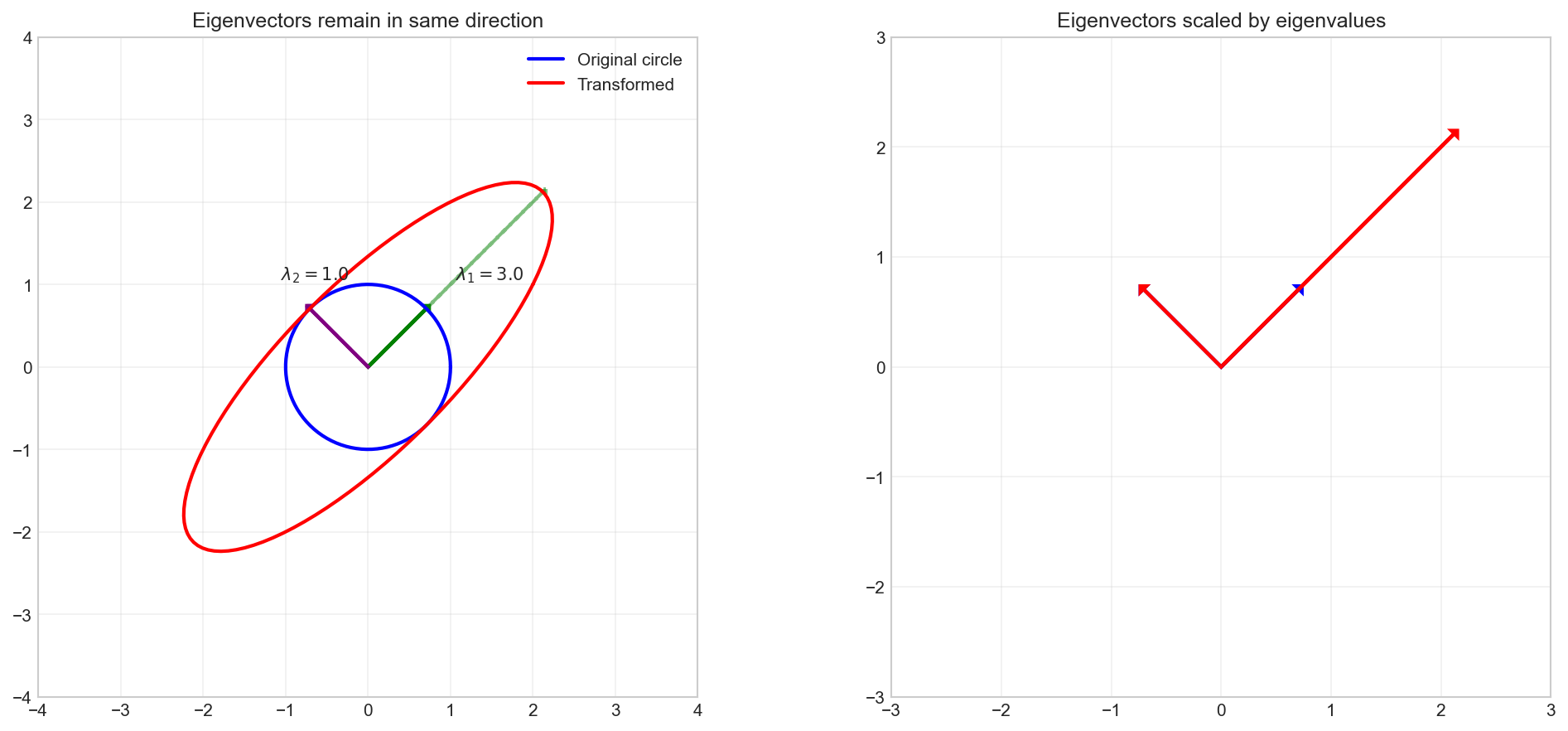
Geometric Interpretation
Let’s visualize how eigenvectors remain in the same direction after transformation:
# Create a matrix with clear eigenvector directions
B = np.array([[2, 1],
              [1, 2]])

eigenvalues_B, eigenvectors_B = np.linalg.eig(B)

fig, axes = plt.subplots(1, 2, figsize=(14, 6))

# Generate a circle of unit vectors
theta = np.linspace(0, 2*np.pi, 100)
circle_x = np.cos(theta)
circle_y = np.sin(theta)
circle = np.vstack([circle_x, circle_y])

# Transform the circle
transformed = B @ circle

# Plot original and transformed
ax1 = axes[0]
ax1.plot(circle_x, circle_y, 'b-', linewidth=2, label='Original circle')
ax1.plot(transformed[0], transformed[1], 'r-', linewidth=2, label='Transformed')

# Plot eigenvectors
colors = ['green', 'purple']
for i in range(2):
    v = eigenvectors_B[:, i]
    lam = eigenvalues_B[i]
    ax1.arrow(0, 0, v[0], v[1], head_width=0.1, head_length=0.05,
              fc=colors[i], ec=colors[i], linewidth=2)
    ax1.arrow(0, 0, lam*v[0], lam*v[1], head_width=0.1, head_length=0.05,
              fc=colors[i], ec=colors[i], linewidth=2, linestyle='--', alpha=0.5)
    ax1.annotate(f'$\\lambda_{i+1}={lam:.1f}$', xy=(v[0]*1.5, v[1]*1.5))

ax1.set_xlim(-4, 4)
ax1.set_ylim(-4, 4)
ax1.set_aspect('equal')
ax1.grid(True, alpha=0.3)
ax1.legend()
ax1.set_title('Eigenvectors remain in same direction')

# Plot eigenvalue scaling
ax2 = axes[1]
for i in range(2):
    v = eigenvectors_B[:, i]
    lam = eigenvalues_B[i]
    ax2.arrow(0, 0, v[0], v[1], head_width=0.08, head_length=0.04,
              fc='blue', ec='blue', linewidth=2, label=f'v_{i+1}' if i==0 else '')
    ax2.arrow(0, 0, lam*v[0], lam*v[1], head_width=0.08, head_length=0.04,
              fc='red', ec='red', linewidth=2, label=f'A*v_{i+1}' if i==0 else '')

ax2.set_xlim(-3, 3)
ax2.set_ylim(-3, 3)
ax2.set_aspect('equal')
ax2.grid(True, alpha=0.3)
ax2.set_title('Eigenvectors scaled by eigenvalues')

plt.tight_layout()
plt.show()

print(f"Eigenvalues: {eigenvalues_B}")
print(f"Eigenvectors:\n{eigenvectors_B}")
Eigenspaces
The eigenspace corresponding to eigenvalue $\lambda$ is the set of all eigenvectors with that eigenvalue, plus the zero vector:
# Find the eigenspace for each eigenvalue
def find_eigenspace(A, eigenvalue):
    """Find a basis for the eigenspace of the given eigenvalue."""
    n = A.shape[0]
    I = np.eye(n)
    B = A - eigenvalue * I

    # The eigenspace is the null space of (A - lambda*I)
    from scipy.linalg import null_space
    return null_space(B)

from scipy.linalg import null_space

print("Eigenspaces for matrix B:")
for i, lam in enumerate(eigenvalues_B):
    eigenspace = find_eigenspace(B, lam)
    print(f"\nEigenvalue lambda = {lam}")
    print(f"Eigenspace basis:\n{eigenspace}")
Eigenspaces for matrix B:

Eigenvalue lambda = 3.0
Eigenspace basis:
[[0.70710678]
 [0.70710678]]

Eigenvalue lambda = 1.0
Eigenspace basis:
[[-0.70710678]
 [ 0.70710678]]
Properties of Eigenvalues
Property 1: Sum of Eigenvalues = Trace
C = np.array([[4, 2, 1],
              [1, 3, 1],
              [2, 1, 5]])

eigenvalues_C, _ = np.linalg.eig(C)

print(f"Matrix C:\n{C}\n")
print(f"Eigenvalues: {eigenvalues_C}")
print(f"Sum of eigenvalues: {np.sum(eigenvalues_C):.6f}")
print(f"Trace of C: {np.trace(C)}")
Matrix C:
[[4 2 1]
 [1 3 1]
 [2 1 5]]

Eigenvalues: [6.79128785 2.79128785 2.41742430]
Sum of eigenvalues: 12.000000
Trace of C: 12
Property 2: Product of Eigenvalues = Determinant
print(f"Product of eigenvalues: {np.prod(eigenvalues_C):.6f}")
print(f"Determinant of C: {np.linalg.det(C):.6f}")
Product of eigenvalues: 45.000000
Determinant of C: 45.000000
Property 3: Eigenvalues of A^n
If $\lambda$ is an eigenvalue of $\boldsymbol{A}$, then $\lambda^n$ is an eigenvalue of $\boldsymbol{A}^n$.
# Compute A^3
A_cubed = np.linalg.matrix_power(A, 3)
eigenvalues_A3, _ = np.linalg.eig(A_cubed)

print(f"Eigenvalues of A: {eigenvalues}")
print(f"Eigenvalues of A^3: {eigenvalues_A3}")
print(f"Original eigenvalues cubed: {eigenvalues**3}")
Eigenvalues of A: [3. 2.]
Eigenvalues of A^3: [27.  8.]
Original eigenvalues cubed: [27.  8.]
Property 4: Eigenvalues of A^(-1)
If $\lambda$ is an eigenvalue of $\boldsymbol{A}$, then $1/\lambda$ is an eigenvalue of $\boldsymbol{A}^{-1}$.
A_inv = np.linalg.inv(A)
eigenvalues_Ainv, _ = np.linalg.eig(A_inv)

print(f"Eigenvalues of A: {eigenvalues}")
print(f"Eigenvalues of A^(-1): {eigenvalues_Ainv}")
print(f"1/eigenvalues: {1/eigenvalues}")
Eigenvalues of A: [3. 2.]
Eigenvalues of A^(-1): [0.33333333 0.5       ]
1/eigenvalues: [0.33333333 0.5       ]
Special Cases
Symmetric Matrices
Symmetric matrices ($\boldsymbol{A} = \boldsymbol{A}^T$) have special properties:
- All eigenvalues are real
- Eigenvectors corresponding to distinct eigenvalues are orthogonal
# Symmetric matrix
S = np.array([[4, 2, 2],
              [2, 5, 1],
              [2, 1, 6]])

eigenvalues_S, eigenvectors_S = np.linalg.eig(S)

print(f"Symmetric matrix S:\n{S}\n")
print(f"Eigenvalues (all real): {eigenvalues_S}\n")
print(f"Eigenvectors:\n{eigenvectors_S}\n")

# Check orthogonality
print("Dot products between eigenvectors:")
for i in range(3):
    for j in range(i+1, 3):
        dot = np.dot(eigenvectors_S[:, i], eigenvectors_S[:, j])
        print(f"  v{i+1} . v{j+1} = {dot:.10f}")
Symmetric matrix S:
[[4 2 2]
 [2 5 1]
 [2 1 6]]

Eigenvalues (all real): [8.04891734 3.64312226 3.30796040]

Eigenvectors:
[[-0.48507125 -0.74230161  0.46225553]
 [-0.53791704  0.66744419  0.51474155]
 [-0.68918137 -0.05992199 -0.72219685]]

Dot products between eigenvectors:
  v1 . v2 = -0.0000000000
  v1 . v3 = 0.0000000000
  v2 . v3 = 0.0000000000
Summary
In this article, we covered:
- Eigenvectors and eigenvalues: $\boldsymbol{A}\vec{v} = \lambda\vec{v}$
- Computing with
np.linalg.eig() - Characteristic polynomial: $\det(\boldsymbol{A} - \lambda\boldsymbol{I}) = 0$
- Geometric interpretation: Eigenvectors define invariant directions
- Eigenspaces: Null space of $(\boldsymbol{A} - \lambda\boldsymbol{I})$
- Properties: trace, determinant, matrix powers
- Symmetric matrices: Real eigenvalues, orthogonal eigenvectors
Resources
Linear Algebra: Python Series - View all articles in this series.
This blog post, titled: "Linear Algebra: Eigenvalues and Eigenvectors Part 1: Linear Algebra Crash Course for Programmers Part 6" by Craig Johnston, is licensed under a Creative Commons Attribution 4.0 International License.
