This article covers solving linear systems in Go using the gonum library, including direct methods with mat.Solve, LU decomposition, and Cholesky decomposition for positive-definite matrices.
Linear Algebra: Golang Series - View all articles in this series.
Previous articles in this series:
This continues from Part 2, linked above.
§2026 Update
The gonum solvers here all still compile and run on current Go: SolveVec, mat.LU, mat.Cholesky, mat.QR, and mat.SVD are unchanged. Two things worth a word.
On the “Go vs Python” framing below: for dense linear algebra, do not expect Go to be dramatically faster than NumPy. Both gonum and NumPy hand the heavy lifting to optimized BLAS and LAPACK routines, so a matrix solve lands in roughly the same place either way. Go’s real advantages here are operational, a single static binary with no interpreter to ship, real concurrency, and easy embedding in a service, not raw FLOPs.
And as in the previous article, this is dense-matrix territory. For large sparse systems the iterative methods in the diagram up top (Conjugate Gradient, GMRES) are what you want, and gonum’s support for them is thin, so that is another point where you may reach past gonum.
The article continues below. The 2026 Update above covers what’s worth knowing today.
§The Linear System Problem
The goal is to solve $\boldsymbol{A}\vec{x} = \vec{b}$ for $\vec{x}$, where $\boldsymbol{A}$ is an $n \times n$ matrix.
§Using mat.Solve
The simplest approach in gonum:
package main

import (
    "fmt"
    "gonum.org/v1/gonum/mat"
)

func main() {
    // System: 2x + 3y = 8
    //         x - y = 1
    A := mat.NewDense(2, 2, []float64{
        2, 3,
        1, -1,
    })
    b := mat.NewVecDense(2, []float64{8, 1})

    // Solve Ax = b
    var x mat.VecDense
    err := x.SolveVec(A, b)
    if err != nil {
        fmt.Printf("Error: %v\n", err)
        return
    }

    fmt.Println("Solution:")
    fmt.Printf("x = %.4f\n", x.AtVec(0))
    fmt.Printf("y = %.4f\n", x.AtVec(1))

    // Verify: A*x should equal b
    var result mat.VecDense
    result.MulVec(A, &x)
    fmt.Printf("\nVerification (A*x): [%.2f, %.2f]\n",
        result.AtVec(0), result.AtVec(1))
}
Output:
Solution:
x = 2.2000
y = 1.2000

Verification (A*x): [8.00, 1.00]
§Visualizing the Solution
A system of two linear equations represents two lines. The solution is their intersection:
package main

import (
    "image/color"

    "gonum.org/v1/plot"
    "gonum.org/v1/plot/plotter"
    "gonum.org/v1/plot/vg"
    "gonum.org/v1/plot/vg/draw"
)

func main() {
    p := plot.New()
    p.Title.Text = "Linear System: Two Lines Intersecting"
    p.X.Label.Text = "x"
    p.Y.Label.Text = "y"
    p.X.Min, p.X.Max = -1, 5
    p.Y.Min, p.Y.Max = -1, 4

    // Line 1: 2x + 3y = 8  =>  y = (8 - 2x) / 3
    line1Pts := make(plotter.XYs, 100)
    for i := range line1Pts {
        x := -1.0 + float64(i)*0.06
        line1Pts[i] = plotter.XY{X: x, Y: (8 - 2*x) / 3}
    }
    l1, _ := plotter.NewLine(line1Pts)
    l1.Color = color.RGBA{R: 66, G: 133, B: 244, A: 255}
    l1.Width = vg.Points(2)

    // Line 2: x - y = 1  =>  y = x - 1
    line2Pts := make(plotter.XYs, 100)
    for i := range line2Pts {
        x := -1.0 + float64(i)*0.06
        line2Pts[i] = plotter.XY{X: x, Y: x - 1}
    }
    l2, _ := plotter.NewLine(line2Pts)
    l2.Color = color.RGBA{R: 234, G: 67, B: 53, A: 255}
    l2.Width = vg.Points(2)

    // Solution point (2.2, 1.2)
    solPts := plotter.XYs{{X: 2.2, Y: 1.2}}
    sol, _ := plotter.NewScatter(solPts)
    sol.GlyphStyle.Color = color.RGBA{R: 52, G: 168, B: 83, A: 255}
    sol.GlyphStyle.Radius = vg.Points(6)
    sol.GlyphStyle.Shape = draw.CircleGlyph{}

    p.Add(l1, l2, sol)
    p.Save(6*vg.Inch, 5*vg.Inch, "systems.png")
}
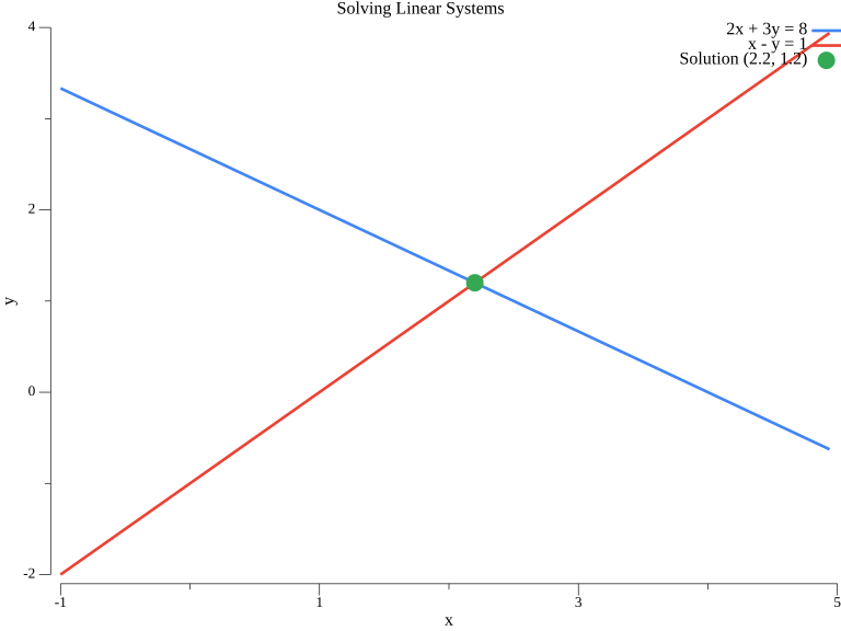
The blue line represents 2x + 3y = 8, the red line represents x - y = 1, and the green point marks the solution (2.2, 1.2).
§LU Decomposition
LU decomposition factors a matrix as $\boldsymbol{A} = \boldsymbol{L}\boldsymbol{U}$ where $\boldsymbol{L}$ is lower triangular and $\boldsymbol{U}$ is upper triangular:
import "gonum.org/v1/gonum/mat"

func luDecomposition() {
    A := mat.NewDense(3, 3, []float64{
        2, -1, 0,
        -1, 2, -1,
        0, -1, 2,
    })

    // Compute LU decomposition
    var lu mat.LU
    lu.Factorize(A)

    // Extract L and U
    var L, U mat.TriDense
    lu.LTo(&L)
    lu.UTo(&U)

    fmt.Println("L (lower triangular):")
    fmt.Printf("%v\n", mat.Formatted(&L))

    fmt.Println("\nU (upper triangular):")
    fmt.Printf("%v\n", mat.Formatted(&U))

    // Solve using LU
    b := mat.NewVecDense(3, []float64{1, 0, 1})
    var x mat.VecDense
    err := lu.SolveVecTo(&x, false, b)
    if err != nil {
        fmt.Printf("Error: %v\n", err)
        return
    }

    fmt.Println("\nSolution x:")
    fmt.Printf("%v\n", mat.Formatted(&x))
}
§Cholesky Decomposition
For symmetric positive-definite matrices, Cholesky decomposition is more efficient: $\boldsymbol{A} = \boldsymbol{L}\boldsymbol{L}^T$
func choleskyDecomposition() {
    // Symmetric positive-definite matrix
    A := mat.NewSymDense(3, []float64{
        4, 2, 2,
        2, 5, 1,
        2, 1, 6,
    })

    // Compute Cholesky decomposition
    var chol mat.Cholesky
    ok := chol.Factorize(A)
    if !ok {
        fmt.Println("Matrix is not positive-definite")
        return
    }

    // Extract L
    var L mat.TriDense
    chol.LTo(&L)

    fmt.Println("Cholesky factor L:")
    fmt.Printf("%v\n", mat.Formatted(&L))

    // Solve using Cholesky
    b := mat.NewVecDense(3, []float64{1, 2, 3})
    var x mat.VecDense
    err := chol.SolveVecTo(&x, b)
    if err != nil {
        fmt.Printf("Error: %v\n", err)
        return
    }

    fmt.Println("\nSolution:")
    fmt.Printf("%v\n", mat.Formatted(&x))
}
§QR Decomposition for Least Squares
For overdetermined systems (more equations than unknowns), use QR decomposition:
func qrLeastSquares() {
    // Overdetermined system: 4 equations, 2 unknowns
    A := mat.NewDense(4, 2, []float64{
        1, 1,
        1, 2,
        1, 3,
        1, 4,
    })
    b := mat.NewVecDense(4, []float64{2.1, 3.9, 6.2, 7.8})

    // QR decomposition
    var qr mat.QR
    qr.Factorize(A)

    // Solve least squares
    var x mat.VecDense
    err := qr.SolveVecTo(&x, false, b)
    if err != nil {
        fmt.Printf("Error: %v\n", err)
        return
    }

    fmt.Println("Least squares solution:")
    fmt.Printf("Intercept: %.4f\n", x.AtVec(0))
    fmt.Printf("Slope: %.4f\n", x.AtVec(1))

    // Compute residuals
    var residuals mat.VecDense
    residuals.MulVec(A, &x)
    residuals.SubVec(&residuals, b)

    residualNorm := mat.Norm(&residuals, 2)
    fmt.Printf("\nResidual norm: %.4f\n", residualNorm)
}
Output:
Least squares solution:
Intercept: 0.1500
Slope: 1.9400

Residual norm: 0.2864
§Benchmarking: Go vs Python
Go typically offers significant performance advantages:
import (
    "fmt"
    "time"
    "gonum.org/v1/gonum/mat"
)

func benchmarkSolve() {
    sizes := []int{100, 500, 1000}

    for _, n := range sizes {
        // Generate random matrix and vector
        data := make([]float64, n*n)
        for i := range data {
            data[i] = float64(i%17) - 8
        }
        A := mat.NewDense(n, n, data)

        bData := make([]float64, n)
        for i := range bData {
            bData[i] = float64(i % 11)
        }
        b := mat.NewVecDense(n, bData)

        // Time the solve
        start := time.Now()
        var x mat.VecDense
        x.SolveVec(A, b)
        elapsed := time.Since(start)

        fmt.Printf("Size %4d x %4d: %v\n", n, n, elapsed)
    }
}
§Condition Number
Check numerical stability by computing the condition number:
func conditionNumber() {
    A := mat.NewDense(3, 3, []float64{
        1, 2, 3,
        4, 5, 6,
        7, 8, 9.0001,  // Nearly singular
    })

    // SVD to compute condition number
    var svd mat.SVD
    svd.Factorize(A, mat.SVDThin)

    values := svd.Values(nil)
    cond := values[0] / values[len(values)-1]

    fmt.Printf("Singular values: %v\n", values)
    fmt.Printf("Condition number: %.2e\n", cond)
}
Output:
Singular values: [16.848158309533105 1.0683452562878242 1.6666990740008272e-05]
Condition number: 1.01e+06
The tiny third singular value relative to the first is what drives the huge condition number, a sign this matrix is nearly singular and that solutions against it will be sensitive to small changes.
§Summary
This article covered:
- Direct solving with
mat.Solve - LU decomposition for general square matrices
- Cholesky decomposition for symmetric positive-definite matrices
- QR decomposition for least squares
- Performance benchmarking
- Condition number for numerical stability
The next article covers eigenvalue problems in Go.
§Resources
§Next: Eigenvalue Problems
Check out the next article in this series, Linear Algebra in Go: Eigenvalue Problems.
Linear Algebra: Golang Series - View all articles in this series.