This article covers statistics and data analysis in Go using gonum/stat and gonum/mat: descriptive statistics, covariance matrices, and correlation analysis.

Linear Algebra: Golang Series - View all articles in this series.

Previous articles in this series:

1. Linear Algebra in Go: Vectors and Basic Operations
2. Linear Algebra in Go: Matrix Fundamentals
3. Linear Algebra in Go: Solving Linear Systems
4. Linear Algebra in Go: Eigenvalue Problems
5. Linear Algebra in Go: SVD and Decompositions

This continues from Part 5: SVD and Decompositions.

§Basic Statistics

The gonum.org/v1/gonum/stat package provides statistical functions:

package main

import (
    "fmt"
    "gonum.org/v1/gonum/stat"
)

func main() {
    data := []float64{2.3, 4.5, 1.2, 7.8, 3.4, 5.6, 9.1, 2.8}

    mean := stat.Mean(data, nil)
    variance := stat.Variance(data, nil)
    stdDev := stat.StdDev(data, nil)

    fmt.Printf("Data: %v\n", data)
    fmt.Printf("Mean: %.4f\n", mean)
    fmt.Printf("Variance: %.4f\n", variance)
    fmt.Printf("Std Dev: %.4f\n", stdDev)

    // Median requires sorted data
    sorted := make([]float64, len(data))
    copy(sorted, data)
    stat.SortWeighted(sorted, nil)
    median := stat.Quantile(0.5, stat.Empirical, sorted, nil)
    fmt.Printf("Median: %.4f\n", median)
}

§Covariance Matrix

Compute the covariance matrix from data:

import (
    "gonum.org/v1/gonum/mat"
    "gonum.org/v1/gonum/stat"
)

func covarianceMatrix(X *mat.Dense) *mat.SymDense {
    rows, cols := X.Dims()

    // Center the data
    means := make([]float64, cols)
    for j := 0; j < cols; j++ {
        col := mat.Col(nil, j, X)
        means[j] = stat.Mean(col, nil)
    }

    centered := mat.NewDense(rows, cols, nil)
    for i := 0; i < rows; i++ {
        for j := 0; j < cols; j++ {
            centered.Set(i, j, X.At(i, j)-means[j])
        }
    }

    // Cov = X^T * X / (n-1)
    cov := mat.NewSymDense(cols, nil)
    for i := 0; i < cols; i++ {
        for j := i; j < cols; j++ {
            colI := mat.Col(nil, i, centered)
            colJ := mat.Col(nil, j, centered)
            covIJ := stat.Covariance(colI, colJ, nil)
            cov.SetSym(i, j, covIJ)
        }
    }

    return cov
}

func covarianceExample() {
    // Sample data: 5 observations, 3 features
    X := mat.NewDense(5, 3, []float64{
        1, 2, 3,
        4, 5, 6,
        2, 3, 4,
        5, 6, 7,
        3, 4, 5,
    })

    cov := covarianceMatrix(X)
    fmt.Println("Covariance matrix:")
    fmt.Printf("%v\n", mat.Formatted(cov))
}

§Visualizing Correlation

Scatter plots with regression lines help visualize relationships between variables:

package main

import (
    "fmt"
    "image/color"
    "math/rand"

    "gonum.org/v1/gonum/stat"
    "gonum.org/v1/plot"
    "gonum.org/v1/plot/plotter"
    "gonum.org/v1/plot/vg"
)

func main() {
    rand.Seed(42)
    p := plot.New()
    p.Title.Text = "Correlation Analysis"
    p.X.Label.Text = "X"
    p.Y.Label.Text = "Y"

    n := 80
    pts := make(plotter.XYs, n)
    xData := make([]float64, n)
    yData := make([]float64, n)

    for i := 0; i < n; i++ {
        x := rand.NormFloat64()*2 + 5
        y := 0.8*x + rand.NormFloat64()*1.5
        pts[i] = plotter.XY{X: x, Y: y}
        xData[i] = x
        yData[i] = y
    }

    scatter, _ := plotter.NewScatter(pts)
    scatter.GlyphStyle.Color = color.RGBA{R: 66, G: 133, B: 244, A: 200}
    scatter.GlyphStyle.Radius = vg.Points(4)

    alpha, beta := stat.LinearRegression(xData, yData, nil, false)
    linePts := plotter.XYs{{X: 0, Y: alpha}, {X: 10, Y: alpha + 10*beta}}
    line, _ := plotter.NewLine(linePts)
    line.Color = color.RGBA{R: 234, G: 67, B: 53, A: 255}
    line.Width = vg.Points(2)

    corr := stat.Correlation(xData, yData, nil)
    p.Add(scatter, line)
    p.Legend.Add(fmt.Sprintf("r = %.2f", corr), scatter)
    p.Legend.Top = true

    p.Save(6*vg.Inch, 5*vg.Inch, "statistics.png")
}

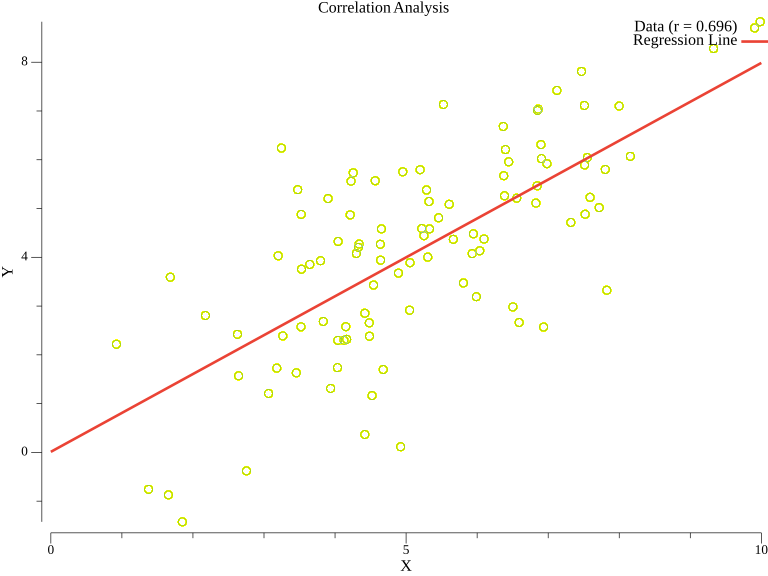
The scatter plot shows the relationship between variables, with the red line representing the linear fit. The correlation coefficient r indicates the strength of the linear relationship.

§Correlation Matrix

Compute Pearson correlation coefficients:

func correlationMatrix(X *mat.Dense) *mat.SymDense {
    _, cols := X.Dims()

    corr := mat.NewSymDense(cols, nil)
    for i := 0; i < cols; i++ {
        for j := i; j < cols; j++ {
            colI := mat.Col(nil, i, X)
            colJ := mat.Col(nil, j, X)
            r := stat.Correlation(colI, colJ, nil)
            corr.SetSym(i, j, r)
        }
    }

    return corr
}

func correlationExample() {
    X := mat.NewDense(100, 3, nil)
    // Generate correlated data
    for i := 0; i < 100; i++ {
        x := float64(i) + rand.NormFloat64()*5
        y := 0.8*x + rand.NormFloat64()*10
        z := rand.NormFloat64() * 20
        X.Set(i, 0, x)
        X.Set(i, 1, y)
        X.Set(i, 2, z)
    }

    corr := correlationMatrix(X)
    fmt.Println("Correlation matrix:")
    fmt.Printf("%v\n", mat.Formatted(corr, mat.Prefix("  ")))
}

§Weighted Statistics

Support for weighted observations:

func weightedStats() {
    data := []float64{1, 2, 3, 4, 5}
    weights := []float64{0.1, 0.2, 0.3, 0.2, 0.2}

    mean := stat.Mean(data, weights)
    variance := stat.Variance(data, weights)

    fmt.Printf("Weighted mean: %.4f\n", mean)
    fmt.Printf("Weighted variance: %.4f\n", variance)
}

§Linear Regression Statistics

func linearRegressionStats() {
    x := []float64{1, 2, 3, 4, 5, 6, 7, 8, 9, 10}
    y := []float64{2.1, 4.2, 5.8, 8.1, 9.9, 12.1, 14.0, 16.2, 17.9, 20.1}

    // Fit linear regression
    alpha, beta := stat.LinearRegression(x, y, nil, false)

    fmt.Printf("y = %.4f + %.4f * x\n", alpha, beta)

    // Compute R-squared
    var ssRes, ssTot float64
    yMean := stat.Mean(y, nil)
    for i := range x {
        pred := alpha + beta*x[i]
        ssRes += (y[i] - pred) * (y[i] - pred)
        ssTot += (y[i] - yMean) * (y[i] - yMean)
    }
    rSquared := 1 - ssRes/ssTot

    fmt.Printf("R-squared: %.4f\n", rSquared)
}

§Summary

This article covered:

• Basic statistics: mean, variance, standard deviation
• Covariance matrix computation
• Correlation matrix using Pearson correlation
• Weighted statistics
• Linear regression with R-squared

§Resources

• Gonum stat Package

Linear Algebra: Golang Series - View all articles in this series.