This article on matrix inverses and determinants is part four of an ongoing crash course on programming with linear algebra, demonstrating concepts and implementations in Python. The inverse of a matrix and the determinant are fundamental concepts that reveal important properties about matrices and provide alternative methods for solving systems of linear equations.
Linear Algebra: Python Series - View all articles in this series.
Previous articles in this series:
This series began with Linear Algebra: Vectors, continued with Linear Algebra: Matrices 1, and most recently covered Systems of Linear Equations.
Python examples in this article make use of the Numpy library. Read the article Python Data Essentials - Numpy if you want a quick overview of this important Python library.
import numpy as np
import matplotlib.pyplot as plt

%matplotlib inline
§The Matrix Inverse
The inverse of a square matrix $\boldsymbol{A}$, denoted $\boldsymbol{A}^{-1}$, is a matrix such that:
Where $\boldsymbol{I}$ is the identity matrix. Not all matrices have inverses; those that do are called invertible or nonsingular.
§Computing the Inverse with NumPy
# Define a 2x2 matrix
A = np.array([[4, 7],
              [2, 6]])

# Compute the inverse
A_inv = np.linalg.inv(A)

print(f"Matrix A:\n{A}\n")
print(f"Inverse A^(-1):\n{A_inv}\n")
Matrix A:
[[4 7]
 [2 6]]

Inverse A^(-1):
[[ 0.6 -0.7]
 [-0.2  0.4]]
# Verify: A @ A^(-1) = I
product = A @ A_inv
print(f"A @ A^(-1):\n{product}\n")

# Check if it's close to identity
identity = np.eye(2)
print(f"Is A @ A^(-1) = I? {np.allclose(product, identity)}")
A @ A^(-1):
[[1. 0.]
 [0. 1.]]

Is A @ A^(-1) = I? True
§Inverse of a 2x2 Matrix
For a 2x2 matrix, the inverse has a closed-form formula:
The term $ad - bc$ is the determinant of the matrix (more on this below).
def inverse_2x2(A):
    """Compute the inverse of a 2x2 matrix manually."""
    a, b = A[0, 0], A[0, 1]
    c, d = A[1, 0], A[1, 1]

    det = a*d - b*c
    if det == 0:
        raise ValueError("Matrix is singular (non-invertible)")

    return np.array([[d, -b],
                     [-c, a]]) / det

# Test the function
A_inv_manual = inverse_2x2(A)
print(f"Manual inverse:\n{A_inv_manual}\n")
print(f"NumPy inverse:\n{A_inv}\n")
print(f"Results match: {np.allclose(A_inv_manual, A_inv)}")
Manual inverse:
[[ 0.6 -0.7]
 [-0.2  0.4]]

NumPy inverse:
[[ 0.6 -0.7]
 [-0.2  0.4]]

Results match: True
§Solving Systems Using the Inverse
If $\boldsymbol{A}\vec{x} = \vec{b}$ and $\boldsymbol{A}$ is invertible, then:
# Solve: 4x + 7y = 22
#        2x + 6y = 14

b = np.array([22, 14])

# Method 1: Using the inverse
x_inverse = A_inv @ b
print(f"Solution using inverse: {x_inverse}")

# Method 2: Using np.linalg.solve (more efficient)
x_solve = np.linalg.solve(A, b)
print(f"Solution using solve:   {x_solve}")

# Verify
print(f"A @ x = {A @ x_inverse}")
Solution using inverse: [1. 2.]
Solution using solve:   [1. 2.]
A @ x = [18. 14.]
Note: While using the inverse works, np.linalg.solve() is preferred for numerical stability and efficiency. Computing the inverse requires more operations and can introduce numerical errors.
§The Determinant
The determinant is a scalar value computed from a square matrix. It encodes important information about the matrix:
- If $\det(\boldsymbol{A}) = 0$, the matrix is singular (non-invertible)
- If $\det(\boldsymbol{A}) \neq 0$, the matrix is invertible
- The absolute value of the determinant represents the scaling factor of the linear transformation
§Determinant of a 2x2 Matrix
# Compute determinant using NumPy
det_A = np.linalg.det(A)
print(f"Matrix A:\n{A}\n")
print(f"Determinant: {det_A}")

# Manual calculation for 2x2
det_manual = A[0,0]*A[1,1] - A[0,1]*A[1,0]
print(f"Manual calculation: {det_manual}")
Matrix A:
[[4 7]
 [2 6]]

Determinant: 10.000000000000002
Manual calculation: 10
§Determinant of a 3x3 Matrix
For a 3x3 matrix, the determinant can be computed using cofactor expansion:
B = np.array([[1, 2, 3],
              [4, 5, 6],
              [7, 8, 9]])

det_B = np.linalg.det(B)
print(f"Matrix B:\n{B}\n")
print(f"Determinant: {det_B:.10f}")
Matrix B:
[[1 2 3]
 [4 5 6]
 [7 8 9]]

Determinant: 0.0000000000
Notice the determinant is essentially zero (numerical precision aside). This means the matrix is singular and cannot be inverted. Let’s verify:
# Check the rank
print(f"Rank of B: {np.linalg.matrix_rank(B)}")
print(f"Matrix B is {'singular' if np.isclose(det_B, 0) else 'invertible'}")

# The rows are linearly dependent: row3 = 2*row2 - row1
print(f"\nRow 3: {B[2]}")
print(f"2*Row2 - Row1: {2*B[1] - B[0]}")
Rank of B: 2
Matrix B is singular

Row 3: [7 8 9]
2*Row2 - Row1: [7 8 9]
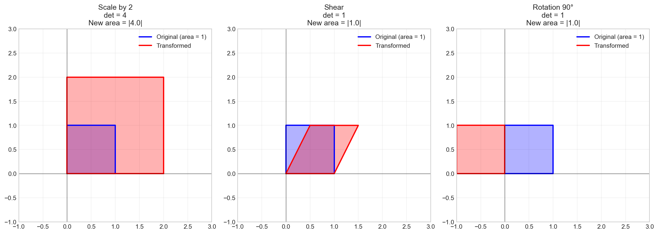
§Geometric Interpretation of the Determinant
The determinant represents how the linear transformation scales areas (in 2D) or volumes (in 3D).
# Visualize the determinant as area scaling
fig, axes = plt.subplots(1, 3, figsize=(15, 5))

# Original unit square
unit_square = np.array([[0, 0], [1, 0], [1, 1], [0, 1], [0, 0]]).T

# Three different transformations
transforms = [
    np.array([[2, 0], [0, 2]]),      # Scale by 2
    np.array([[1, 0.5], [0, 1]]),    # Shear
    np.array([[0, -1], [1, 0]])      # Rotation 90 degrees
]
titles = ['Scale by 2\ndet = 4', 'Shear\ndet = 1', 'Rotation 90°\ndet = 1']

for ax, T, title in zip(axes, transforms, titles):
    # Plot original unit square
    ax.plot(unit_square[0], unit_square[1], 'b-', linewidth=2,
            label='Original (area = 1)')
    ax.fill(unit_square[0], unit_square[1], alpha=0.3, color='blue')

    # Transform the square
    transformed = T @ unit_square
    ax.plot(transformed[0], transformed[1], 'r-', linewidth=2,
            label=f'Transformed')
    ax.fill(transformed[0], transformed[1], alpha=0.3, color='red')

    det = np.linalg.det(T)
    ax.set_title(f'{title}\nNew area = |{det:.1f}|')
    ax.set_xlim(-1, 3)
    ax.set_ylim(-1, 3)
    ax.set_aspect('equal')
    ax.grid(True, alpha=0.3)
    ax.legend()
    ax.axhline(y=0, color='k', linestyle='-', alpha=0.3)
    ax.axvline(x=0, color='k', linestyle='-', alpha=0.3)

plt.tight_layout()
plt.show()
§Properties of Determinants
Determinants have several important properties:
# Create two invertible matrices
A = np.array([[3, 1], [2, 4]])
B = np.array([[1, 2], [3, 1]])

det_A = np.linalg.det(A)
det_B = np.linalg.det(B)

print(f"det(A) = {det_A:.4f}")
print(f"det(B) = {det_B:.4f}")
det(A) = 10.0000
det(B) = -5.0000
§Property 1: det(AB) = det(A) * det(B)
det_AB = np.linalg.det(A @ B)
print(f"det(AB) = {det_AB:.4f}")
print(f"det(A) * det(B) = {det_A * det_B:.4f}")
print(f"Equal: {np.isclose(det_AB, det_A * det_B)}")
det(AB) = -50.0000
det(A) * det(B) = -50.0000
Equal: True
§Property 2: det(A^T) = det(A)
det_AT = np.linalg.det(A.T)
print(f"det(A^T) = {det_AT:.4f}")
print(f"det(A) = {det_A:.4f}")
print(f"Equal: {np.isclose(det_AT, det_A)}")
det(A^T) = 10.0000
det(A) = 10.0000
Equal: True
§Property 3: det(A^(-1)) = 1/det(A)
A_inv = np.linalg.inv(A)
det_A_inv = np.linalg.det(A_inv)
print(f"det(A^(-1)) = {det_A_inv:.4f}")
print(f"1/det(A) = {1/det_A:.4f}")
print(f"Equal: {np.isclose(det_A_inv, 1/det_A)}")
det(A^(-1)) = 0.1000
1/det(A) = 0.1000
Equal: True
§Property 4: det(cA) = c^n * det(A) for n x n matrix
c = 3
n = 2  # 2x2 matrix
det_cA = np.linalg.det(c * A)
print(f"det({c}A) = {det_cA:.4f}")
print(f"{c}^{n} * det(A) = {(c**n) * det_A:.4f}")
print(f"Equal: {np.isclose(det_cA, (c**n) * det_A)}")
det(3A) = 90.0000
3^2 * det(A) = 90.0000
Equal: True
§Cramer’s Rule
Cramer’s Rule provides an explicit formula for solving systems of linear equations using determinants. For a system $\boldsymbol{A}\vec{x} = \vec{b}$:
Where $\boldsymbol{A}_i$ is the matrix $\boldsymbol{A}$ with its $i$-th column replaced by $\vec{b}$.
def cramers_rule(A, b):
    """Solve Ax = b using Cramer's Rule."""
    det_A = np.linalg.det(A)
    if np.isclose(det_A, 0):
        raise ValueError("Matrix is singular; Cramer's Rule not applicable")

    n = len(b)
    x = np.zeros(n)

    for i in range(n):
        A_i = A.copy()
        A_i[:, i] = b  # Replace i-th column with b
        x[i] = np.linalg.det(A_i) / det_A

    return x

# Solve the system:
# 3x + y = 9
# 2x + 4y = 14

A = np.array([[3, 1],
              [2, 4]])
b = np.array([9, 14])

# Using Cramer's Rule
x_cramer = cramers_rule(A, b)
print(f"Cramer's Rule solution: {x_cramer}")

# Verify with np.linalg.solve
x_solve = np.linalg.solve(A, b)
print(f"np.linalg.solve:        {x_solve}")
Cramer's Rule solution: [2. 3.]
np.linalg.solve:        [2. 3.]
Note: While Cramer’s Rule is elegant, it’s computationally expensive for large systems. It’s mainly useful for theoretical analysis and small systems.
§Properties of Invertible Matrices
A square matrix $\boldsymbol{A}$ is invertible if and only if:
- $\det(\boldsymbol{A}) \neq 0$
- $\boldsymbol{A}$ has full rank ($rank(\boldsymbol{A}) = n$)
- The columns (or rows) of $\boldsymbol{A}$ are linearly independent
- The system $\boldsymbol{A}\vec{x} = \vec{b}$ has exactly one solution for every $\vec{b}$
- The null space of $\boldsymbol{A}$ contains only the zero vector
# Check various properties for an invertible matrix
C = np.array([[1, 2, 3],
              [0, 1, 4],
              [5, 6, 0]])

print(f"Matrix C:\n{C}\n")
print(f"Determinant: {np.linalg.det(C):.4f}")
print(f"Rank: {np.linalg.matrix_rank(C)}")
print(f"Is invertible: {not np.isclose(np.linalg.det(C), 0)}")
Matrix C:
[[1 2 3]
 [0 1 4]
 [5 6 0]]

Determinant: 1.0000
Rank: 3
Is invertible: True
# Compute and display the inverse
C_inv = np.linalg.inv(C)
print(f"Inverse of C:\n{C_inv}\n")

# Verify
print(f"C @ C^(-1):\n{np.round(C @ C_inv, 10)}")
Inverse of C:
[[-24.  18.   5.]
 [ 20. -15.  -4.]
 [ -5.   4.   1.]]

C @ C^(-1):
[[1. 0. 0.]
 [0. 1. 0.]
 [0. 0. 1.]]
§Numerical Considerations
When working with matrix inverses and determinants in practice, numerical precision matters:
# Create a nearly singular matrix
D = np.array([[1, 2],
              [1.0001, 2.0002]])

det_D = np.linalg.det(D)
print(f"Matrix D:\n{D}\n")
print(f"Determinant: {det_D}")
print(f"Condition number: {np.linalg.cond(D):.2f}")
Matrix D:
[[1.     2.    ]
 [1.0001 2.0002]]

Determinant: 1.9999999899641377e-08
Condition number: 60003750.03
The condition number indicates how sensitive the solution is to small changes in the input. A large condition number suggests the matrix is ill-conditioned.
# Solving with an ill-conditioned matrix can give unreliable results
b1 = np.array([3, 3.0003])
b2 = np.array([3, 3.0004])  # Small change in b

x1 = np.linalg.solve(D, b1)
x2 = np.linalg.solve(D, b2)

print(f"Solution for b1: {x1}")
print(f"Solution for b2: {x2}")
print(f"Change in b: {np.linalg.norm(b2 - b1):.6f}")
print(f"Change in x: {np.linalg.norm(x2 - x1):.2f}")
Solution for b1: [1. 1.]
Solution for b2: [-3999. 2001.]
Change in b: 0.000100
Change in x: 5000.00
§Summary
In this article, we covered:
- Matrix inverse: $\boldsymbol{A}^{-1}$ such that $\boldsymbol{A}\boldsymbol{A}^{-1} = \boldsymbol{I}$
- Computing inverses with
np.linalg.inv() - Determinants and their geometric interpretation as scaling factors
- Properties of determinants: multiplicative, transpose invariance, etc.
- Cramer’s Rule for solving systems using determinants
- Invertibility conditions and their equivalence
- Numerical considerations for ill-conditioned matrices
§Resources
- Matrix Inverse - Khan Academy
- Determinants - Khan Academy
- NumPy Linear Algebra
- Condition Number - Wikipedia
§Next: Vector Spaces and Subspaces
Check out the next article in this series, Linear Algebra: Vector Spaces and Subspaces.
Linear Algebra: Python Series - View all articles in this series.